AIM: To create and study the Mass scaling factor for both Implicit and Explicit methods for calculating and reducing the Runtime and Stability of the model in Mass Scaling.
Objective:
Mass Scaling:
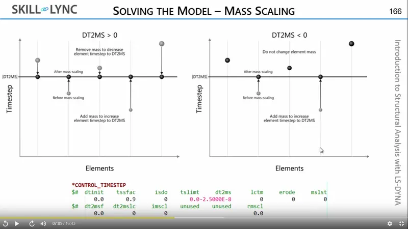
When DT2MS is input as a negative value, mass is added only to those elements whose timestep would otherwise be less than
|DT2MS|. By adding mass to these elements, their timestep becomes equal to |DT2MS|. An infinite number of combinations of TSSFAC and DT2MS will give the same product, i.e., timestep but the added mass will be different for each combination. The trend is that the bigger |DT2MS| (and the smaller TSSFAC while TSSFAC*|DT2MS|=const), the greater the added mass. In return, stability may improve as TSSFAC is reduced (just as in non-mass-scaled solutions). If stability is a problem with the default TSSFAC of 0.9, try 0.8 or 0.7. If you reduce TSSFAC, you can increase |DT2MS| proportionally so that their product, and hence timestep, is unchanged.
To determine where and when mass is automatically added, write GLSTAT and MATSUM files. These files will allow you to plot added mass vs. time for the complete model and individual parts. To produce fringe plots of added mass in parts comprised of shell elements (DT2MS negative), set STSSZ=3 in *DATABASE_EXTENT_BINARY. You can then fringe the added mass (per element) using LS-POST by choosing Fcomp > Misc > time step size. (Here, the label "time step size" is the element added mass.)
The hard limit on mass scaling is 8% and stability should be completely intact. This means that two simulations, one with mass scaling and one without should behave the same way. To contain the trials for mass scaling and the data generated henceforth. Both the DT and TSSFAC parameters should be optimized. And to take the attached model and do trial and error for mass scaling. Once the mass scaling objective is reached, a histogram should be plotted to compare the runtime with mass scaling trials. Finally, run the same model using an implicit solver with necessary changes and compare implicit and explicit runtime. And to understand mass scaling parameters.
As per Courant-Friedrich's condition for explicit analysis is

where Δt is the timestep, emin, min is the size of the smallest mesh element and C is the speed of the stress wave.
The scaling factor is used for providing numerical stability to the solution.
Also,
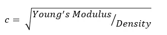
If we increase the density of small elements, we get an increased timestep. Henceforth, reducing the solution run time.
Without mass scaling:
Firstly, the simulation is set to run in the LS-DYNA manager without any mass scaling parameters to know the default computational time.
With Constant TSSFAC = 0.9
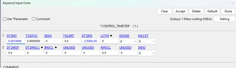
Case 1(i) :
Here the Value of the DT2MS is changed to -0.000035, with TSSFAC as 0.9
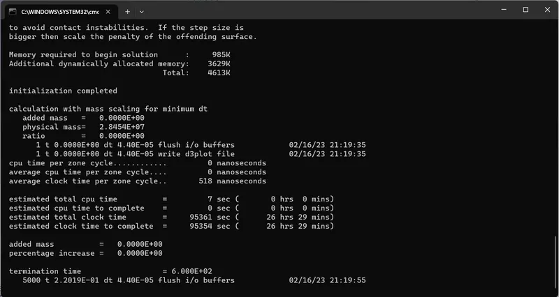
LS- Run:
From the below result the Added mass = 0, and Physical mass = 2.84e+7; Ratio of Added to the Physical mass = 0;
The Whole simulation is taken 26hrs to complete the simulation, so we have to change the DT2MS the reduce of Simulation timing and get rid of the stability
Here the Value of No mass is Added to the Component, therefore the value of DT is -4.4e-5 so we have to consider higher the value of what we obtained now.
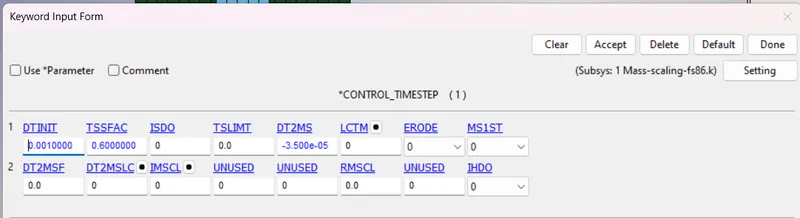
Case 1 (ii):
Here the Value of the DT2MS is changed to -0.000035, with TSSFAC as 0.9
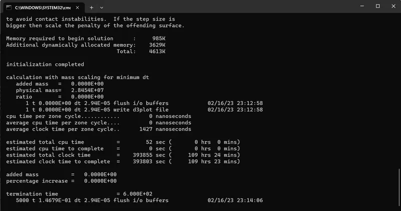
LS-Run:
The multiple of TSSFAC and DT2MS is what we get as DT here 2.94e-5
The only difference between the previous case of TSSFAC is an increase in Simulation time but the Mass Scaling remains as Case 2(I) of 4.84%
So that increase in hours is 109hrs 23mins.
Mass scaling procedure in LS-DYNA:
LS-DYNA allows two different types of mass scaling using the DT2MS parameter from *CONTROL_TIMESTEP with the default set to no mass scaling.
When DT2MS is less than zero, LS-DYNA adds the mass of each element whose timestep is below abs(DT2MS) such that the element's updated DT is equal to abs(DT2MS).
When DT2MS is more significant than zero, LS-DYNA adds mass to elements whose DT is below abs(DT2MS) and "removes" mass from elements whose DT is more significant than zero.
DT2MS > 0 is seldom used while DTM2S < 0 is frequently used for overcoming the smallest computed timestep.
Care must be taken when using DT2MS < 0 to ensure that the added mass does not hurt the simulation accuracy
In this project work, the simulation is carried out initially without mass scaling to find the default computational time, then by varying the mass scaling parameters to reduce the simulation run time.
Case 2 (i) :
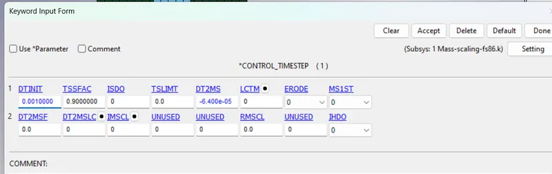
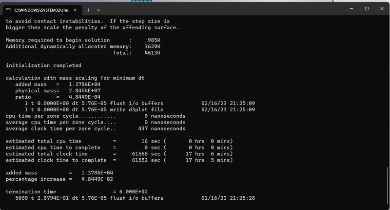
Here the Value of the DT2MS is changed to -0.000064, with TSSFAC as 0.9
LS-Run:
Here slight change occurs and a Change in a mass of 0.048% is insufficient because we need 8% of mass scaling added to the component.
So changes need to be done.
Case 2 (ii):
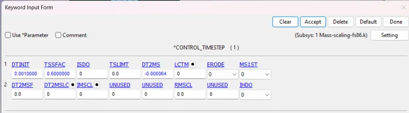
Here the Value of the DT2MS is changed to -0.000064, with TSSFAC as 0.6
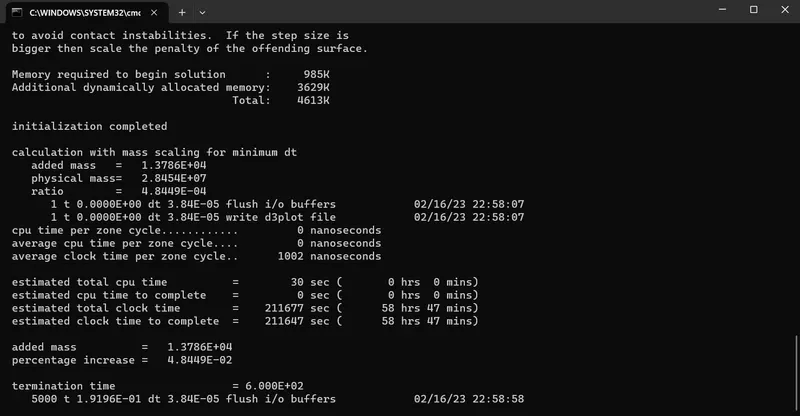
LS-Run:
The multiple of TSSFAC and DT2MS is what we get as DT here 3.84e-5
The only difference between the previous case of TSSFAC is an increase in Simulation time but the Mass Scaling remains as Case 2(I) of 4.84%
So that increase in hours is 58hrs 47mins
Case 3 (i):
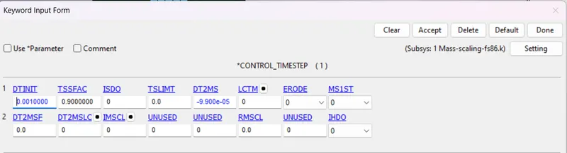
Here the Value of the DT2MS is changed to -0.000099, with TSSFAC as 0.9
LS-RUN:
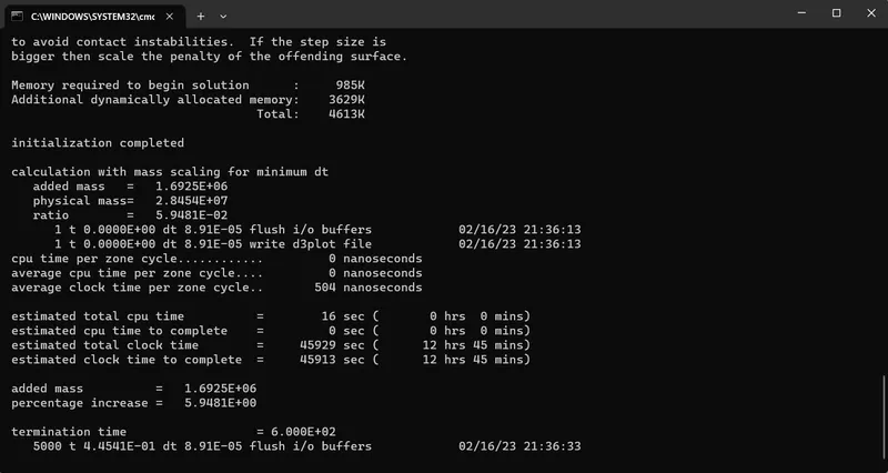
Added mass = 1.69e+6 , physical mass = 2.84e+7, Ratio = 5.94e-2;
Here the Run time is getting lesser as compared to the previous case, the Simulation time is approx 12hrs 45mins.
But the Mass Changing is near 8% but not 8%, so re-run the model by changing the value of DT2MS and run the simulation.
Case 3 (ii):
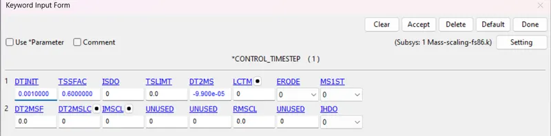
Here the Value of the DT2MS is changed to -0.000099, with TSSFAC as 0.6
LS-Run:
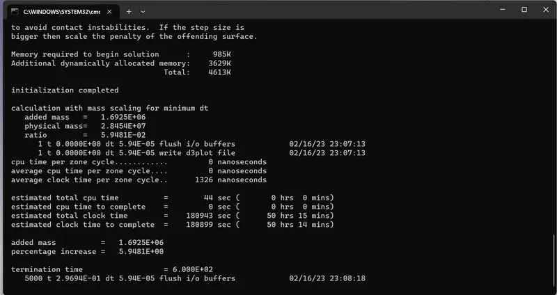
The multiple of TSSFAC and DT2MS is what we get as DT here 5.94e-5
The only difference between the previous case of TSSFAC is an increase in Simulation time but the Mass Scaling remains as Case 3(I) of 5.94%
So that increase in hours is 50hrs 15mins
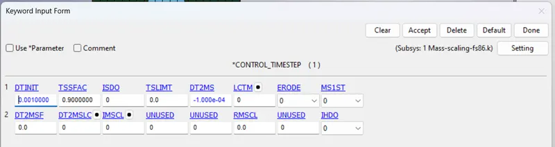
Case 4 (i) :
Here the Value of the DT2MS is changed to -0.0001, with TSSFAC as 0.9
LS-Run:
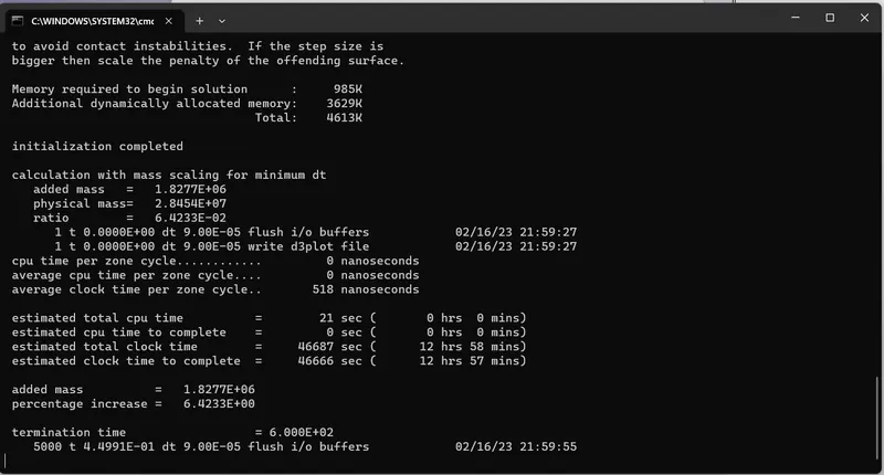
Added Mass = 1.82e+6; Physical mass = 2.84e+7; Ratio = 6.42e-2;
Here the run for the Simulation has been reduced to 12hrs 58mins, but the mass scaling is 6.43%, but we can get up to 8%, let us try another simulation to check whether we can get it.
Case 4(ii):
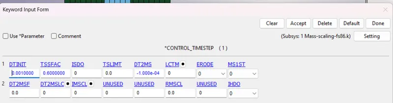
Here the Value of the DT2MS is changed to -0.0001, with TSSFAC as 0.6
LS-RUN:
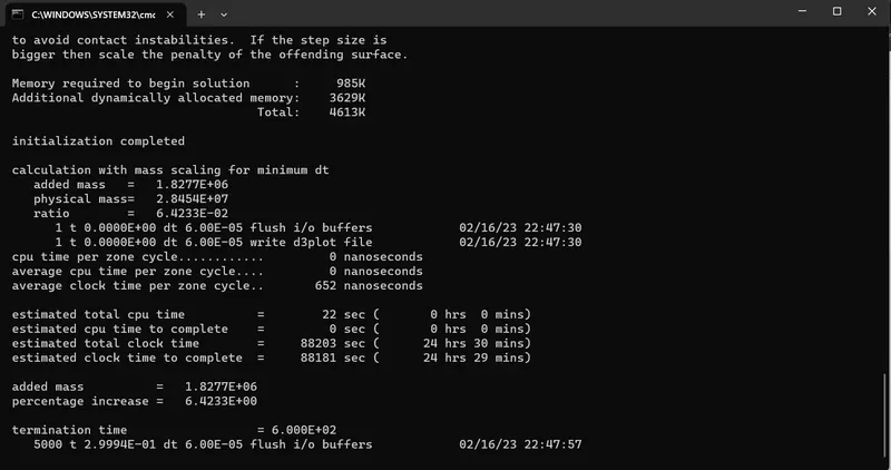
The multiple of TSSFAC and DT2MS is what we get as DT here 6e-5
The only difference between the previous case of TSSFAC is an increase in Simulation time but the Mass Scaling remains as Case 5(I) of 6.43%
So that increase in hours is 24hrs 30mins
Case 5 (i):
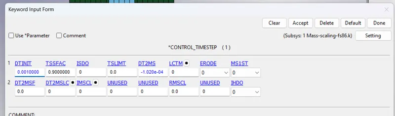
Here the Value of the DT2MS is changed to -0.000102, with TSSFAC as 0.9
LS-Run:
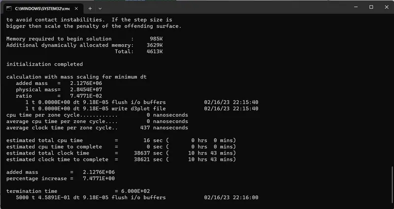
Added Mass = 2.12e+6; Physical mass = 2.84e+7; Ratio = 7.47e-2;
Here the run for the Simulation has been decreased from the previous to 10hrs 30mins, but the mass scaling is 7.47%, but we can get up to 8%, let us try another simulation to check whether we can get it.
Case 5(ii):
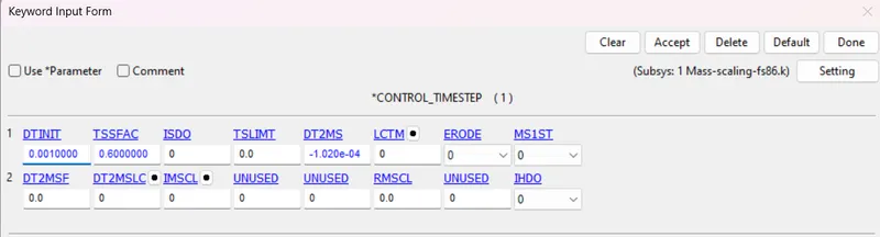
Here the Value of the DT2MS is changed to -0.000102, with TSSFAC as 0.6
LS-Run:
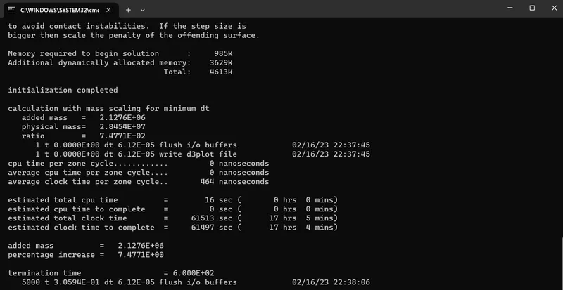
Added Mass = 2.12e+6; Physical mass = 2.84e+7; Ratio = 7.47e-2;
The only difference between the previous case of TSSFAC is an increase in Simulation time but the Mass Scaling remains as Case 5(I) of 7.47%
So that increase in hours is 17hrs 5mins
CASE 6(i):
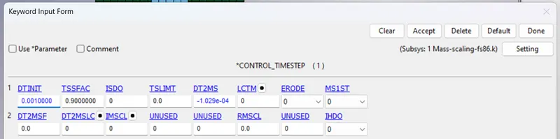
Here the Value of the DT2MS is changed to -0.0001029, with TSSFAC as 0.9
LS-Run:
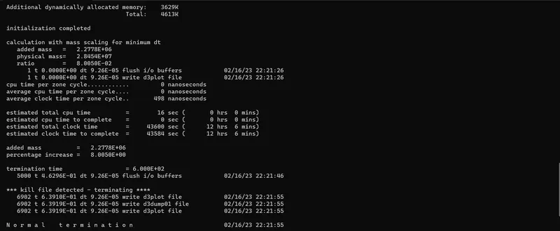
Added Mass = 2.77e+6; Physical mass = 2.84e+7; Ratio = 8.005e-2;
Here we have got the 8% of Mass scaling, so we have achieved the Mass scaling.
Case 6(ii):
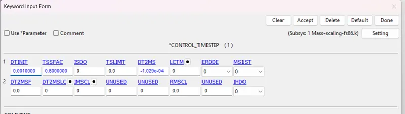
TSSFAC = 0.6, DT2MS = 0.0001029;
LS-Run:
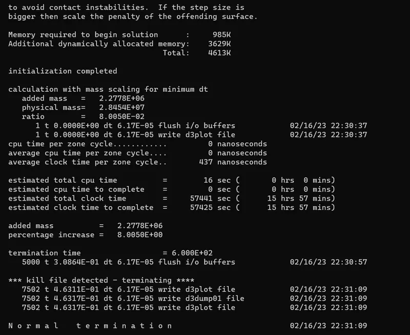
Here the DT is set to 6.17e-5, as the TSSFAC is set to 0.6
Here we have got the 8% of Mass scaling, so we have achieved the Mass scaling.
The only difference between the previous case of TSSFAC is an increase in Simulation time but the Mass Scaling remains as Case 6(I) of 6.43%
So that increase in hours is 15hrs 57mins.
As we assign Two different scenarios such as:
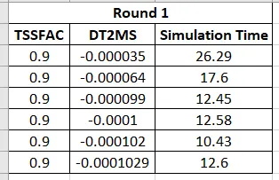
Round 1:
With TSSFAC is 0.9 and DT2MS changed as shown in the table.
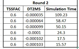
Round 2:
With TSSFAC is 0.6 and DT2MS changed as shown in the table.
Comparatively from both case, the Mass scaling is similar by the Total simulation time is getting differ a lot in TSSFAC 0.6 and 0.9
From this Case Study, I have learned that 0.9 of TSSFAC and perfect DT2MS will give Accurate results.
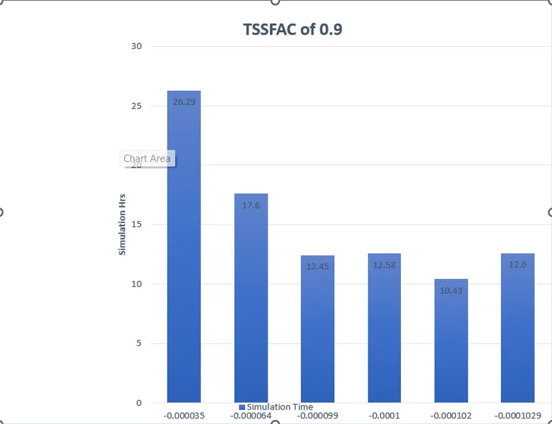
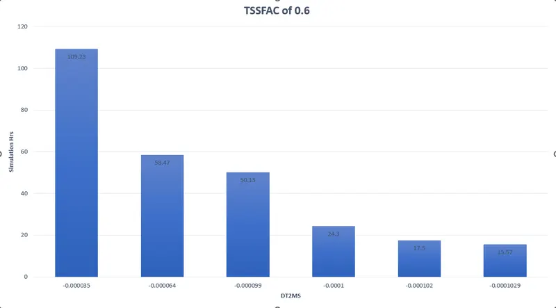
Histogram:
TSSFAC of 0.9
TSSFAC of 0.6:
Procedure:
Implicit Simulation:
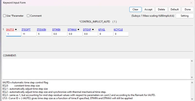
In Implicit simulation here we import the model, and then to run the implicit model we need a Basic Control card such as Implicit General and Implicit Auto card
1) CONTROL_IMPLICIT_AUTO
Keyword manager -> CONTROL -> IMPLICIT_AUTO KEYWORD.
CONTROL_IMPLICIT_AUTO card is used for automatic time step control during implicit analysis.
The input value for the Automatic time step control flag = IAUTO = 1.
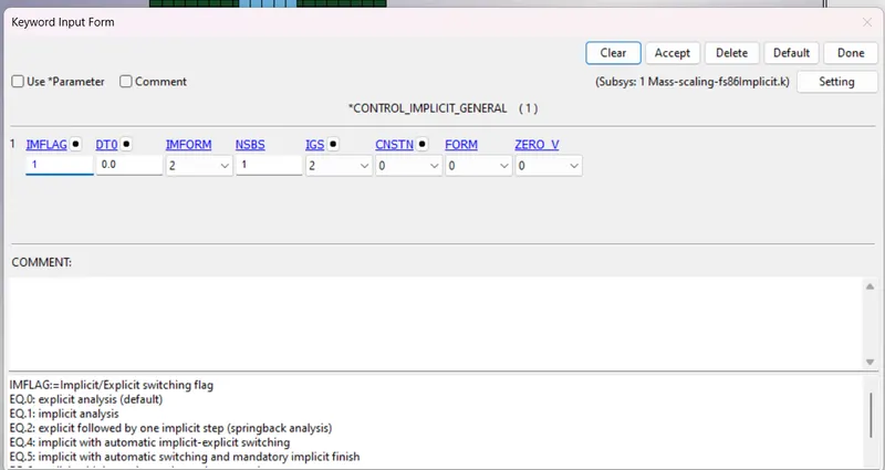
CONTROL IMPLICIT_GENERAL:
KEYWORD CONTROL_IMPLICIT_GENERAL card activates implicit analysis and defines associated control parameters. This keyword is required for all implicit analyses. The input value for IMFLAG=Implicit/Explicit switching flag = 1 (implicit analysis) DT0=Initial time step size for implicit analysis.
LS_RUN:
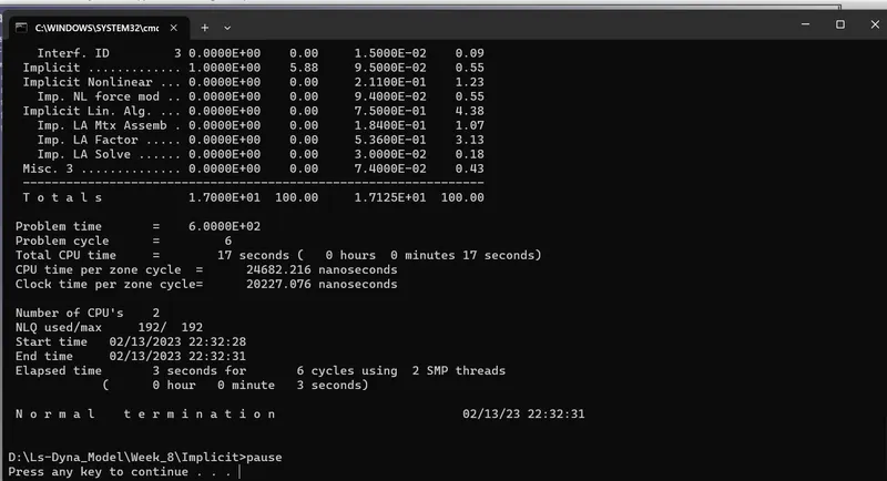
The whole simulation is not taken more than 5ms, since it is an Implicit method, then meantime for the whole simulation will be lesser and so it takes only 3ms
LS-Post processing:
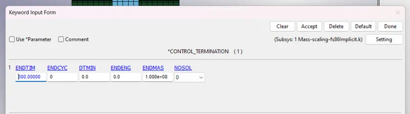
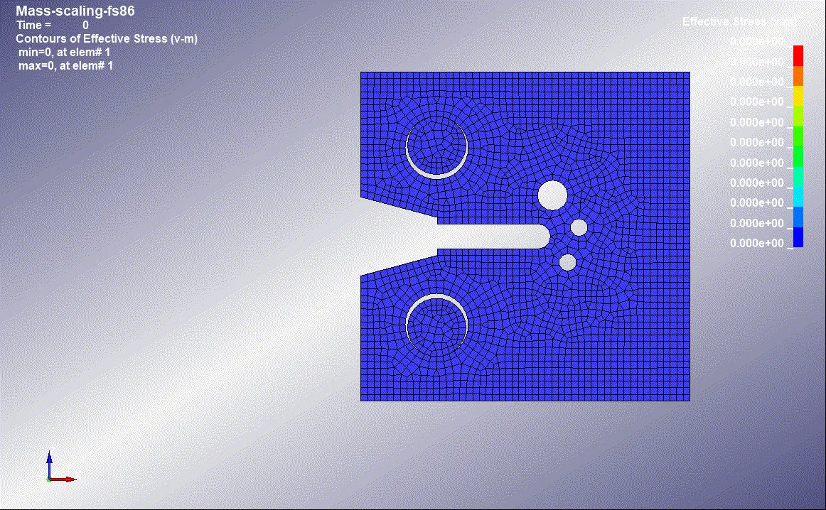
Here the maximum Stress occurs at 2.76e-6 N-mm^2, for the 3ms of termination, and Termination is considered as 600 ms.
Conclusion:
i) Mass-scaling is a term used for scaling the element's mass in explicit simulations to adjust its timestep.
ii) The primary motivation is to increase the global compute timestep which is limited by the Courant's stability criteria.
iii) Implicit and Explicit analysis differs in the approach to time increments.
iv) In Implicit analysis, each time increment has to converge, but we can set pretty long time increments. Explicit on the other hand doesn’t have to converge each increment, but for the solution to be accurate time increments must be super small.
v) Both implicit and explicit analysis do more or less the same thing. They divide the analysis time into small increments and then analyze what is going on in our model one increment after another.
vi) The speed of computing is exactly the difference between implicit and explicit.
vii) Though the running time for implicit analysis is shorter than the explicit analysis method, the debate on what type of solver is better depends upon the type of problem and accuracy we need.
viii) Through the Simulation study for Explicit with Change in TSSFAC results in an increase in Simulation timing but mass Scaling values remain same for the both the case of TSSFAC.