REYNOLDS-AVERAGED NAVIER–STOKES(RANS) EQUATIONS AND ITS ANALYSIS
The objective of this project is to apply Reynold's decomposition to the Navier-Stokes equation and to determine the expression for Reynold's Stress.
Navier Stokes Equations:
The movement of fluid in the physical domain is driven by various properties. For the purpose of bringing the behavior of fluid flow to light and developing a mathematical model, those properties have to be defined precisely as to provide the transition between the physical and the numerical derivation. Velocity, pressure, temperature, density, and viscosity are the main properties that should be considered simultaneously when conducting the fluid flow examination. In accordance with the physical incidents such as combustion, multiphase flow, turbulence, mass transport, etc., those properties diversify enormously, which can be categorized into kinematic, transport, thermodynamic, and other properties.
It is relatively easy, for instance, to solve these equations for a flow between parallel plates or for the flow in a circular pipe. For more complex geometries, however, the equations need to be resolved depending upon the flow regime of interest, it is often possible to simplify these equations. In other cases, additional equations may be required. In the field of fluid dynamics, the different flow regimes are categorized using a non-dimensional number such as the Reynolds number and the Mach number.
All the governing equations are based on the laws of conservation. The Navier- Stokes equations are applied to a mathematical model to examine changes in those properties during dynamic or thermal interactions. The equations are adjustable regarding the content of the problem and are expressed based on the principles of conservation of mass, momentum, and energy.
Turbulence
"Turbulence is an irregular motion which in general makes its appearance in fluids, gaseous or liquid, when they flow past solid surfaces or even when neighboring streams of the same fluid flow past or over one another. "
Turbulence is a continuous phenomenon that exists on a large range of length and time scales, which are still larger than molecular scales. In order to visualize turbulent flows, one often refers to turbulent eddies, which can be thought of as a local swirling motion whose characteristic dimension is on the order of the local turbulence length scale. Turbulent eddies also overlap in space, where larger eddies carry smaller ones. As there exists a large range of different scales (or turbulent eddy sizes), an energy cascade exists by which energy is transferred from the larger scales to the smaller scales, and eventually to the smallest scales where the energy is dissipated into heat by molecular viscosity.
Turbulent flows are thus always dissipative.Turbulent flows also exhibit a largely enhanced diffusivity. This turbulent diffusion greatly enhances the transfer of mass, momentum, and energy. The apparent stresses, therefore, may be of several orders of magnitude greater than in the corresponding laminar case. The fact that the Navier-Stokes equations are non-linear for turbulent flows leads to interactions
between fluctuations of different wavelengths and directions. The wavelengths of the motion may be as large as a characteristic scale on the order of the width of the flow, all the way to the smallest scales, which are limited by the viscous dissipation of energy. The action of vortex stretching is mainly responsible for spreading the motion over a wide range of wavelengths.
Wavelengths which are nearly comparable to the characteristic mean-flow scales interact most strongly with the mean flow. This implies that the larger-scale turbulent eddies are most responsible for the energy transfer and enhanced diffusivity. In turn, these large eddies cause random stretching of the vortex elements of the smaller eddies, and energy is cascades down from the largest to the smallest scales.
Direct Numerical Simulation:
Numerical methods that do not employ any averaging and turbulent models – known as Direct Numerical Simulation (DNS) have been developed. The DNS does not depend on any turbulent model (often empirical) and are based on the local instantaneous governing equations. The DNS is the closest to the real transport phenomena, but it is computationally most intensive. Since DNS is not practical for many engineering problems, alternative approaches like Reynolds Averaged Numerical Solution (RANS) or Large Eddy Simulation (LES) can be employed. For academic research, on the other hand, DNS can reproduce experimental resolution for experiments that are either very difficult or impossible. With advancements on parallel computing, one can break up the computational task and set to multiple CPUs to perform computation simultaneously. The scale of the number of grid points required for a DNS to capture the physics of the simplest turbulent flow is
`N approx L/eta`
where, L is the length scale of the largest turbulent eddy
`eta` is the length scale of the viscous effects.
The length scale of viscous effect is also referred as Komogorov Scale, and is given as:
`eta = (nu^3/(epsi))^(1/4)`
where `nu` is the kinematic viscosity and `sigma` is the rate of kinetic energy dissipation. It has been shown that the scale of `L/eta` is:
`N ~ L/eta ~ (Re_L)^(3/4)`
where `Re_L` is the turbulent Reynolds number.
When DNS is employed to solve a three-dimensional turbulent problem, the number of grid required will be:
`N^3~(Re_L)^(9/4)`
which shows that the DNS can easily run into computational limitation of speed and memory for large Reynolds numbers. Nevertheless, significant progresses have been made in DNS of turbulent flow especially turbulent boundary layer structures.
Turbulence is the state of chaotic and unstable fluid flow, just opposite of Laminar flow. Y plus(Y+) is the non-dimensional distance of the first cell from the wall.
Let's takes an example of a flat plate under zero pressure gradient and front left side the uniform velocity is coming to the plate. Firstly, it will be laminar flow, then after some disturbance, the region will be called as Transition Region, when the disturbance is growing too much the flow will change in Turbulent Flow. The boundary layer in the turbulent region will be called a turbulent boundary layer whereas in laminar it will be called the laminar boundary layer.
Reynold's Number `Re` is the ratio of Inertial force to the Viscous Force.
`Re=frac{rho*V*l}{mu}`
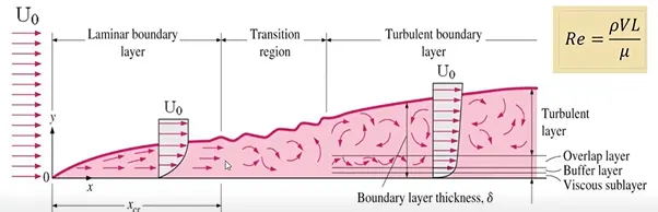
External Flow :Re<`5x10^5` Laminar Flow || Re>`5x10^5` Turbulent Flow
Internal Flow :Re<`2300` Laminar Flow || Re>`4000` Turbulent Flow
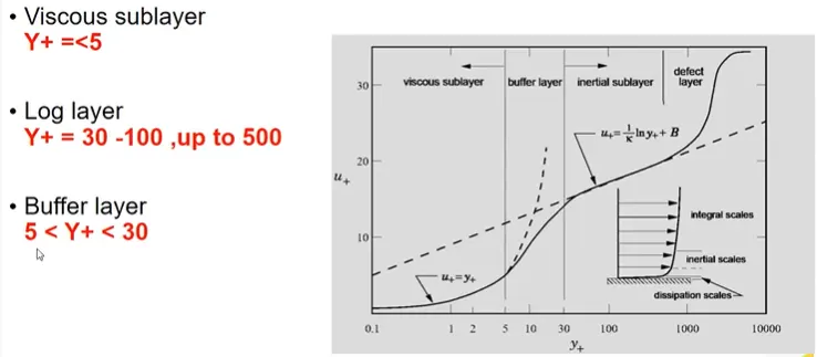
Viscous Sub Layer: Viscous stress term dominates
Buffer Layer: Transitional region
Log law Region: Reynolds shear stress term dominates
Reynold's Stress
In fluid dynamics, the Reynolds stress is the component of the total stress tensor in a fluid obtained from the averaging operation over the Navier-Stokes equations to account for turbulent fluctuations in fluid momentum.
Turbulence Modeling Approaches
Converge offers two turbulence modeling approaches
-Reynold-Averaged Navier Stokes (RANS)-Solves equation for an ensemble-averaged velocity field and the magnitude of the turbulent fluctuations.
-Large Eddy Simulation (LES)-Solves equations for a filtered time-dependent velocity field that represents large scale turbulence motion
Governing Equations for incompressible flow:
Continuity Equation - Conservation of Mass:
`(∂u)/(∂x)+(∂v)/(∂y)=0`
x-Momentum Equation - Conservation of Momentum ( Newton's Second law):
`ρ[(∂u)/(∂t)+u(∂u)/(∂x)+v(∂u)/(∂y)]=-(∂P)/(∂x)+ μ ((∂^2u)/(∂x^2)+(∂^2u)/(∂y^2))`
Energy/Transport Equation - Conservation of Energy ( First law of thermodynamics):
`ρC_P[(∂ϕ)/(∂t)+u(∂ϕ)/(∂x)+v(∂ϕ)/(∂y)]=K[ (∂^2ϕ)/(∂x^2)+(∂^2ϕ)/(∂y^2)]+μ ((∂u)/(∂y))^2`
Reynolds-averaged Navier Stokes Equations (RANS) :
Although statistical theory and numerical simulation (DNS) are viable options, most of the research on turbulent flow analysis in the past century has used the concept of time averaging. Applying the time averaging to the basic equations of motion yields the Reynolds equations, which involve both mean and fluctuating quantities. One then attempts to model the fluctuation terms by relating them to mean properties or their gradients. This approach may now be yielding diminishing returns. Lumley (1989) gives a stimulating discussion of how time averaging might outlive its usefulness. The Reynolds equations are far from obsolete, however, and form the basis of most engineering analyses of turbulent flow.
Need of RANS:
Most of the engineering simulations need to be computationally effective (less computational effort). To capture the minute effects of turbulence DNS cannot be applied effectively (high computation effort required) and it requires the mesh size to be of order (1e-9 or less) to be in compliance with CFL number and small-time steps, it is going to be computationally inviable. Hence, to be computationally viable, engineers depend upon the time-averaged solutions, where the turbulence of engineering needs is captured effectively. Here the time step used is large compared to the relevant period of fluctuations of components. Hence a coarse grid than the one used for DNS can be used which will reduce the computational effort.
Reynolds Decomposition:
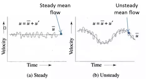
Following the idea of Reynolds (1895), we assume that the fluid is in a random unsteady turbulent state and work with the time-averaged or mean equations of motion. Any variable 'Q' is resolved into a mean value of `barQ`plus a fluctuating value Q', where by definition,
`barQ = 1/T int_(t_0)^(t_0+T)Q dt`
Instantaneous quantity at any point in space and time = Time-averaged Quantity + Fluctuating component.
where T is large compared to the relevant period of fluctuations. The mean value `barQ`itself may vary slowly with time as shown in the image below.
Let us consider only incompressible turbulent flow with constant transport properties but with possible significant fluctuations in velocity, pressure, and temperature.
`u(x,y,t) = baru(x,y)+u'(x,y,t)`
`v(x,y,t) = barv(x,y)+v'(x,y,t)`
`P(x,y,t) = barP(x,y)+P'(x,y,t)`
`T(x,y,t) = barT(x,y)+T'(x,y,t)`
`ϕ(x,y,t) = bar ϕ(x,y)+ϕ'(x,y,t)`
Time averaged quantities:
`barQ(x,y) = 1/T int_(t_0)^(t_0+T)Q(x,y,t) dt`
mean values are not the function of 't' .
Moreover, the averaging of fluctuating terms lead to zero as shown below.
`1/Tint_0^Tu(x,y,t) dt= 1/Tint_0^Tbaru(x,y)dt+1/Tint_0^Tu'(x,y,t)dt`
and
`1/Tint_0^Tu(x,y,t) dt= baru(x,y)`
`1/Tint_0^Tbaru(x,y)dt = baru(x,y)`
implies
`int_0^Tu'(x,y,t)dt = 0`
Before substituting these functions in the NS equations, we can verify from basic integral relation that the following rules of averaging apply for any two turbulent quantities 'f' and 'g'.
`bar(f') = 0`
`bar(barf)=barf`
`bar(fbarg)=barfbarg`
`bar(f'barg) = 0`
`bar(f+g) = barf+barg`
`bar(∂f)/(∂s) = (∂barf)/(∂s)`
`bar(fg)=barfbarg+bar(f'g')`
`bar(intfds) = intbarf ds`
Substituting Averged quantites in NS-equations:
Contnuity Equation:
`(∂u)/(∂x)+(∂v)/(∂y)=0`
substituting the averaged quantities
`(∂(baru+u'))/(∂x)+(∂(barv+v'))/(∂y)=0`
expanding the terms
`(∂baru)/(∂x)+(∂u')/(∂x)+(∂barv)/(∂y)+(∂v')/(∂y)=0`
averaging over time step 'T'
`1/Tint_0^T(∂baru)/(∂x)dt+1/Tint_0^T(∂u')/(∂x)dt+1/Tint_0^T(∂barv)/(∂y)dt+1/Tint_0^T(∂v')/(∂y)dt=0`
since the time integral of fluctuation component is zero and integral limit not a function of space.
`1/Tint_0^T(∂baru)/(∂x)dt+color(red)cancel(1/Tint_0^T(∂u')/(∂x)dt)+1/Tint_0^T(∂barv)/(∂y)dt+color(red)cancel(1/Tint_0^T(∂v')/(∂y)dt)=0`
The
equation reduces to
`1/Tint_0^T(∂baru)/(∂x)dt+1/Tint_0^T(∂barv)/(∂y)dt=0`
since the `baru` and `barv` is the function of space only, the above equation can be re-written as:
`(∂baru)/(∂x)1/Tint_0^Tdt+(∂barv)/(∂y)1/Tint_0^Tdt=0`
and
`1/Tint_0^Tdt=(T-0)/T = 1`
implies, the continuity equation after the substitution of averaged quantities depends on only mean values of decomposed quantities as shown below.
`color(red)((∂baru)/(∂x)+(∂barv)/(∂y)=0`
x-Momentum Equation:
`ρ[(∂u)/(∂t)+u(∂u)/(∂x)+v(∂u)/(∂y)]=-(∂P)/(∂x)+ μ ((∂^2u)/(∂x^2)+(∂^2u)/(∂y^2))`
multiplying both sides by `1/ρ` and replacing `μ/ρ` with kinematic viscosity `nu`
`(∂u)/(∂t)+u(∂u)/(∂x)+v(∂u)/(∂y)=-1/rho(∂P)/(∂x)+ ν (∂^2u)/(∂x^2)+ ν (∂^2u)/(∂y^2)`
to convert the above equation in suitable form, we multiply x-component of velocity with continuity equation and add it to left hand side and its resultant is zero.
`(∂u)/(∂t)+u(∂u)/(∂x)+v(∂u)/(∂y)+u((∂u)/(∂x)+(∂v)/(∂y))=-1/rho(∂P)/(∂x)+ ν (∂^2u)/(∂x^2)+ ν (∂^2u)/(∂y^2)`
rearranging the terms in the above equation
`(∂u)/(∂t)+2u(∂u)/(∂x)+v(∂u)/(∂y)+u(∂v)/(∂y)=-1/rho(∂P)/(∂x)+ ν (∂^2u)/(∂x^2)+ ν (∂^2u)/(∂y^2)`
From Product rule
`(∂(uv))/(∂y) =u(∂v)/(∂y)+v(∂u)/(∂y)`
and
`2u(∂u)/(∂x) = (∂u^2)/(∂x)`
substituting the terms of product rule in the reduced equation.
`(∂u)/(∂t)+(∂u^2)/(∂x)+(∂(uv))/(∂y)=-1/rho(∂P)/(∂x)+ ν (∂^2u)/(∂x^2)+ ν (∂^2u)/(∂y^2)`
substituting the averaged quantities
`(∂(baru+u'))/(∂t)+(∂(baru+u')^2)/(∂x)+(∂((baru+u')(barv+v')))/(∂y)=-1/rho(∂(barP+P'))/(∂x)+ ν (∂^2(baru+u'))/(∂x^2)+ ν (∂^2(baru+u'))/(∂y^2)`
expanding the terms
`(∂baru)/(∂t)+(∂u')/(∂t)+(∂baru^2)/(∂x)+(∂(u')^2)/(∂x)+(∂(2baru u'))/(∂x)+(∂(barubarv))/(∂y)+(∂(baru v'))/(∂y)+(∂(u'barv))/(∂y)+(∂(u'v'))/(∂y)=-1/rho(∂barP)/(∂x)-1/rho(∂P')/(∂x)+ ν (∂^2baru)/(∂x^2)+ ν (∂^2u')/(∂x^2)+ ν (∂^2baru)/(∂y^2)+ ν (∂^2u')/(∂y^2)`
averaging over time step T
`1/Tint_0^T(∂baru)/(∂t)dt+1/Tint_0^T(∂u')/(∂t)dt+1/Tint_0^T(∂baru^2)/(∂x)dt+1/Tint_0^T(∂(u')^2)/(∂x)dt+1/Tint_0^T(∂(2baru u'))/(∂x)dt+1/Tint_0^T(∂(barubarv))/(∂y)dt+1/Tint_0^T(∂(baru v'))/(∂y)dt+1/Tint_0^T(∂(u'barv))/(∂y)dt+1/Tint_0^T(∂(u'v'))/(∂y)dt=-1/Tint_0^T1/rho(∂barP)/(∂x)dt-1/Tint_0^T1/rho(∂P')/(∂x)dt+ 1/Tint_0^Tν (∂^2baru)/(∂x^2)dt+ 1/Tint_0^Tν (∂^2u')/(∂x^2)dt+ 1/Tint_0^Tν (∂^2baru)/(∂y^2)dt+ 1/Tint_0^Tν (∂^2u')/(∂y^2)dt`
since the time integral of fluctuation component is zero and the rules mentioned above.
`1/Tint_0^T(∂baru)/(∂t)dt+color(red)cancel(1/Tint_0^T(∂u')/(∂t)dt)+1/Tint_0^T(∂baru^2)/(∂x)dt+1/Tint_0^T(∂(u')^2)/(∂x)dt+color(red)cancel(1/Tint_0^T(∂(2baru u'))/(∂x)dt)+1/Tint_0^T(∂(barubarv))/(∂y)dt+color(red)cancel(1/Tint_0^T(∂(baru v'))/(∂y)dt)+color(red)cancel(1/Tint_0^T(∂(u'barv))/(∂y)dt)+1/Tint_0^T(∂(u'v'))/(∂y)dt=-1/Tint_0^T1/rho(∂barP)/(∂x)dt-color(red)cancel(1/Tint_0^T1/rho(∂P')/(∂x)dt)+ 1/Tint_0^Tν (∂^2baru)/(∂x^2)dt+ color(red)cancel(1/Tint_0^Tν (∂^2u')/(∂x^2)dt)+ 1/Tint_0^Tν (∂^2baru)/(∂y^2)dt+ color(red)cancel(1/Tint_0^Tν (∂^2u')/(∂y^2)dt)`
The above equation reduces to
`1/Tint_0^T(∂baru)/(∂t)dt+1/Tint_0^T(∂baru^2)/(∂x)dt+1/Tint_0^T(∂(u')^2)/(∂x)dt+1/Tint_0^T(∂(barubarv))/(∂y)dt+1/Tint_0^T(∂(u'v'))/(∂y)dt=-1/Tint_0^T1/rho(∂barP)/(∂x)dt+ 1/Tint_0^Tν (∂^2baru)/(∂x^2)dt+ 1/Tint_0^Tν (∂^2baru)/(∂y^2)dt`
Upon integrating, the equation reduces to
`(∂baru)/(∂t)+(∂baru^2)/(∂x)+1/Tint_0^T(∂(u')^2)/(∂x)dt+(∂(barubarv))/(∂y)+1/Tint_0^T(∂(u'v'))/(∂y)dt=-1/rho(∂barP)/(∂x)+ ν (∂^2baru)/(∂x^2)+ ν (∂^2baru)/(∂y^2)`
Rearranging the terms
`(∂baru)/(∂t)+(∂baru^2)/(∂x)+(∂(barubarv))/(∂y)=-1/rho(∂barP)/(∂x)+ ν (∂^2baru)/(∂x^2)+ ν (∂^2baru)/(∂y^2)-color(red)(1/Tint_0^T(∂(u'v'))/(∂y)dt)-color(red)(1/Tint_0^T(∂(u')^2)/(∂x)dt)`
From the above equation it is clear that the momentum equation obtained with mean values of components is similar to momentum equation of actual transport properties except with the red terms.
If we consider that the `u'` value is fluctuating between -1 and 1 then by averaging it the value of `u'` comes equal to 0 but if we consider the same case for `(u')^2`then the square of -1 and 1 will be between 0 and 1 which when integrated will not give zero. Hence,
`1/Tint_0^T(∂(u')^2)/(∂x)dt !=0`
Moreover, the above term can be approximated to zero in the boundary layer where the gradient along y is higher in comparison to the x-direction. Though we are not using this assumption in this case.
Similarly in the term `1/Tint_0^T(∂(u'v'))/(∂y)dt` the fluctuations along the x-axis `u'` and the fluctuations along the y-axis `v'` are correlated. That is when a low momentum y-component is flowing in the positive y-direction then the high momentum (i.e., high velocity) x-component gets slowed down which is caused by `v'`. So, the positive increase in the `v'` is going to cause a negative result in the `u'`, and the product of two will come out to be negative value only. Hence, this term will also not give zero.
`ubrace(color(blue)((∂baru)/(∂t)))_("change w.r.t time")+ubrace(color(green)((∂baru^2)/(∂x)+(∂(barubarv))/(∂y)))_("convective terms")=ubrace(color(violet)(-1/rho(∂barP)/(∂x)))_("Pressure Gradient")+ ubrace(ν ((∂^2baru)/(∂x^2)+(∂^2baru)/(∂y^2)))_("Shear Stress")-ubrace(color(red)(1/Tint_0^T(∂(u'v'))/(∂y)dt)-color(red)(1/Tint_0^T(∂(u')^2)/(∂x)dt))_("Reynolds Stress")`
In the above equation, integral values are replaced by averages.
`(∂baru)/(∂t)+(∂baru^2)/(∂x)+(∂(barubarv))/(∂y)=-1/rho(∂barP)/(∂x)+ ν (∂^2baru)/(∂x^2)+ ν (∂^2baru)/(∂y^2)-(∂(bar(u'v')))/(∂y)-(∂(bar((u')^2)))/(∂x)`
The equation can be further rearranged as follows:
`(∂baru)/(∂t)+(∂baru^2)/(∂x)+(∂(barubarv))/(∂y)=-1/rho(∂barP)/(∂x)+ ν (∂^2baru)/(∂x^2)+ ν (∂^2baru)/(∂y^2)+1/ρ[(∂(-ρbar(u'v')))/(∂y)+(∂(-ρbar((u')^2)))/(∂x)]`
In the compact notation:
`"Stress term" = color(blue)(ubrace(μ∇^2u_i)_("shear stress gradient"))-color(red)(ubrace(ρ(∂bar(u_i^')bar(u_j^'))/(∂x_j))_("Reynolds Stress gradient")`
`= μ∂/(∂x_j)((∂u_i)/(∂x_j))-ρ∂/(∂ x_j)(bar(u_i^')bar(u_j^'))`
`= ∂/(∂x_j)[μ((∂u_i)/(∂x_j))-ρ(bar(u_i^')bar(u_j^'))]`
`"Total Shear Stress" = ubrace(μ((∂u_i)/(∂x_j)))_("Laminar Stress")-ubrace(ρ(bar(u_i^')bar(u_j^')))_("Turbulent Stress")`
In the 3D cartesian cordinate system the above equation will be as follows:
`(∂baru)/(∂t)+(∂baru^2)/(∂x)+(∂(barubarv))/(∂y)+(∂(barubarw))/(∂z)=-1/rho(∂barP)/(∂x)+ ν [(∂^2baru)/(∂x^2)+(∂^2baru)/(∂y^2)+(∂^2baru)/(∂z^2)]+1/ρ[(∂(-ρbar((u')^2)))/(∂x)+(∂(-ρbar(u'v')))/(∂y)+(∂(-ρbar(u'w')))/(∂z)]`
Hence the resulting Reynolds stress in the matrix form, along the x, y, and z axes is as follows:
`τ_(ij)^(Reynolds) = [[τ_(x x), τ_(xy), τ_(xz) ],[τ_(yx), τ_(yy), τ_(yz) ],[τ_(zx), τ_(zy), τ_(zz) ]]=[[-ρbar((u')^2),-ρbar((u'v')),-ρbar((u'w'))], [-ρbar((v'u')),-ρbar((v')^2),-ρbar((v'w'))], [-ρbar((w'u')),-ρbar((w'v')),-ρbar((w')^2)]]`
Reynolds stress is a component of stress tensor in fluid which is obtained by averaging operation over the Navier Stokes equation used to account for turbulent fluctuation in the fluid.
Turbulent Viscosity is a function of fluctuations in velocity and is influenced by the randomness of flow. It is non-linear and difficult to estimate. It depends upon flow regimes and is not a property. It is dominant in turbulent flow regimes with high Reynolds numbers.
Molecular Viscosity is a resistance to the movement of one layer of fluid over the adjacent layer. It is linear and easy to measure. It is the fluid property and independent of geometry.
Essentially, the ratio of turbulent to molecular viscosity gives an indication of how strong the Reynolds stresses are, as compared to molecular stresses. So it sounds reasonable to use this ratio as a measure of turbulence. Typically, an eddy viscosity ratio of more than 100 to 1000 indicates a turbulent flow. Although, the evolution of turbulence models has revolved around the definition of eddy viscosity, and hence for different models may have different values of it.
Transport Equation:
`ρC_P[(∂ϕ)/(∂t)+u(∂ϕ)/(∂x)+v(∂ϕ)/(∂y)]=K[ (∂^2ϕ)/(∂x^2)+(∂^2ϕ)/(∂y^2)]+μ ((∂u)/(∂y))^2`
substituting the decomposed forms of the quantities.
`ρC_P[(∂(barϕ+ϕ'))/(∂t)+(baru+u')(∂(barϕ+ϕ'))/(∂x)+(barv+v')(∂(barϕ+ϕ'))/(∂y)]=K[ (∂^2(barϕ+ϕ'))/(∂x^2)+(∂^2(barϕ+ϕ'))/(∂y^2)]+μ ((∂(baru+u'))/(∂y))^2`
Expanding each term
`ρC_P[(∂(barϕ))/(∂t)+(∂(ϕ'))/(∂t)+baru(∂barϕ)/(∂x)+baru(∂ϕ')/(∂x) +u'(∂barϕ)/(∂x) +u'(∂ϕ')/(∂x)+barv(∂barϕ)/(∂y)+barv(∂ϕ')/(∂y) +v'(∂barϕ)/(∂y) +v'(∂ϕ')/(∂y)]=K[ (∂^2barϕ)/(∂x^2)+(∂^2ϕ')/(∂x^2)+(∂^2barϕ)/(∂y^2)+(∂^2ϕ')/(∂y^2)]+μ[ ((∂baru)/(∂y))^2+((∂u')/(∂y))^2+2(∂baru)/(∂y)(∂u')/(∂y)]`
averaging over time step T
`ρC_P[1/Tint_0^T(∂(barϕ))/(∂t)dt+1/Tint_0^T(∂(ϕ'))/(∂t)dt+1/Tint_0^Tbaru(∂barϕ)/(∂x)dt+1/Tint_0^Tbaru(∂ϕ')/(∂x) dt+1/Tint_0^Tu'(∂barϕ)/(∂x) dt+1/Tint_0^Tu'(∂ϕ')/(∂x)dt+1/Tint_0^Tbarv(∂barϕ)/(∂y)dt+1/Tint_0^Tbarv(∂ϕ')/(∂y) dt+1/Tint_0^Tv'(∂barϕ)/(∂y) dt+1/Tint_0^Tv'(∂ϕ')/(∂y)dt]=K[ 1/Tint_0^T(∂^2barϕ)/(∂x^2)dt+1/Tint_0^T(∂^2ϕ')/(∂x^2)dt+1/Tint_0^T(∂^2barϕ)/(∂y^2)dt+1/Tint_0^T(∂^2ϕ')/(∂y^2)dt]+μ[ 1/Tint_0^T((∂baru)/(∂y))^2dt+1/Tint_0^T((∂u')/(∂y))^2dt+1/Tint_0^T2(∂baru)/(∂y)(∂u')/(∂y)dt]`
From the above rules of integrals, many terms gets cancelled out.
`ρC_P[1/Tint_0^T(∂(barϕ))/(∂t)dt+color(red)cancel(1/Tint_0^T(∂(ϕ'))/(∂t)dt)+1/Tint_0^Tbaru(∂barϕ)/(∂x)dt+color(red)cancel(1/Tint_0^Tbaru(∂ϕ')/(∂x) dt)+color(red)cancel(1/Tint_0^Tu'(∂barϕ)/(∂x) dt)+1/Tint_0^Tu'(∂ϕ')/(∂x)dt+1/Tint_0^Tbarv(∂barϕ)/(∂y)dt+color(red)cancel(1/Tint_0^Tbarv(∂ϕ')/(∂y) dt)+color(red)cancel(1/Tint_0^Tv'(∂barϕ)/(∂y) dt)+1/Tint_0^Tv'(∂ϕ')/(∂y)dt]=K[ 1/Tint_0^T(∂^2barϕ)/(∂x^2)dt+color(red)cancel(1/Tint_0^T(∂^2ϕ')/(∂x^2)dt)+1/Tint_0^T(∂^2barϕ)/(∂y^2)dt+color(red)cancel(1/Tint_0^T(∂^2ϕ')/(∂y^2)dt)]+μ[ 1/Tint_0^T((∂baru)/(∂y))^2dt+1/Tint_0^T((∂u')/(∂y))^2dt+color(red)cancel(1/Tint_0^T2(∂baru)/(∂y)(∂u')/(∂y)dt)]`
reduced equation is of form
`ρC_P[1/Tint_0^T(∂(barϕ))/(∂t)dt+1/Tint_0^Tbaru(∂barϕ)/(∂x)dt+1/Tint_0^Tu'(∂ϕ')/(∂x)dt+1/Tint_0^Tbarv(∂barϕ)/(∂y)dt+1/Tint_0^Tv'(∂ϕ')/(∂y)dt]=K[ 1/Tint_0^T(∂^2barϕ)/(∂x^2)dt+1/Tint_0^T(∂^2barϕ)/(∂y^2)dt]+μ[ 1/Tint_0^T((∂baru)/(∂y))^2dt+1/Tint_0^T((∂u')/(∂y))^2dt]`
obtaining the averaged terms
`ρC_P[(∂barϕ)/(∂t)dt+baru(∂barϕ)/(∂x)+color(red)(1/Tint_0^Tu'(∂ϕ')/(∂x)dt)+barv(∂barϕ)/(∂y)+color(red)(1/Tint_0^Tv'(∂ϕ')/(∂y)dt)]=K[ (∂^2barϕ)/(∂x^2)+(∂^2barϕ)/(∂y^2)]+μ[ ((∂baru)/(∂y))^2+color(red)(1/Tint_0^T((∂u')/(∂y))^2dt)]`
From the above equation it is clear that the transport equation obtained with mean values of components is similar to transport equation of actual transport properties except with the red terms.
Replacing the integral terms by average values.
`ρC_P[(∂barϕ)/(∂t)+baru(∂barϕ)/(∂x)+color(red)(bar(u'(∂(ϕ'))/(∂x)))+barv(∂barϕ)/(∂y)+color(red)(bar(v'(∂(ϕ'))/(∂y)))]=K[ (∂^2barϕ)/(∂x^2)+(∂^2barϕ)/(∂y^2)]+μ[ ((∂baru)/(∂y))^2+color(red)(((∂bar(u'))/(∂y))^2)]`
adding the LHS of below term in LHS of the above equation.
`bar(ϕ'(∂(u'))/(∂x))+bar(ϕ'(∂(v'))/(∂y)) = 0`
`ρC_P[(∂barϕ)/(∂t)+baru(∂barϕ)/(∂x)+bar(u'(∂(ϕ'))/(∂x))+barv(∂barϕ)/(∂y)+bar(v'(∂(ϕ'))/(∂y))+color(red)([bar(ϕ'(∂(u'))/(∂x))+bar(ϕ'(∂(v'))/(∂y))])]=K[ (∂^2barϕ)/(∂x^2)+(∂^2barϕ)/(∂y^2)]+μ[ ((∂baru)/(∂y))^2+((∂bar(u'))/(∂y))^2]`
From Product rule the above equation can be reduced to
`ρC_P[(∂barϕ)/(∂t)+baru(∂barϕ)/(∂x)+barv(∂barϕ)/(∂y)+(∂(bar(u'ϕ')))/(∂x)+(∂(bar(v'ϕ')))/(∂y)]=K[ (∂^2barϕ)/(∂x^2)+(∂^2barϕ)/(∂y^2)]+μ[ ((∂baru)/(∂y))^2+((∂bar(u'))/(∂y))^2]`
The extra terms appearing on left hand side are marked in red (i.e., turbulent flux) and on RHS it is turbulent stress dissipation marked in blue.
`ρC_P[(∂barϕ)/(∂t)+baru(∂barϕ)/(∂x)+barv(∂barϕ)/(∂y)+underbrace(color(red)((∂(bar(u'ϕ')))/(∂x)+(∂(bar(v'ϕ')))/(∂y)))_("turbulent flux")]=K[ underbrace(color(green)((∂^2barϕ)/(∂x^2)+(∂^2barϕ)/(∂y^2)))_("molecular flux")]+underbrace(color(purple)(μ((∂baru)/(∂y))^2))_("viscous stress dissipation")+underbrace(color(blue)(μ((∂bar(u'))/(∂y))^2))_("turbulent stress dissipation")`
`underbraceq_("total flux")=underbrace(-k(∂barϕ)/(∂x))_("molecular flux")-underbrace(ρC_Pbar(u'ϕ'))_("turbulent flux")`
In order to model the above transport equation using RANS, we need to figure out on the turbulent flux terms rest of the terms are dependent on the average time scales being used.
The above RANS modeled NS-equations contain many new unknowns involving time-mean correlations of fluctuating velocities and temperature. Therefore solutions cannot be attempted without additional relations or empirical modeling ideas. The above forms the basis for the modeling of any available time averaging turbulence models viz., (k-`ε`, k-`ω` etc.,)