Week 8: Literature review - RANS derivation and analysis
Apply reynold's decomposition to the NS equations and come up with the expression for reynold's stress.
- Explain your understanding of the terms reynold's stress
- What is turbulent viscosity? How is it different from molecular viscosity?
SOLUTION
Aim:
To derive the Reynolds Averaged Navir Stokes(RANS) Equations.
Objective:
To find the expressions for Reynolds stress by applying Reynolds decomposition to the Navier-Stokes equations. Also understanding the difference between the turbulent viscosity and molecular velocity.
Literature Review:
The fluid flow is basically divided into three types i.e. Laminar flow, Transient flow, and Turbulence flow. Generally, the flow can be determined using Reynolds Number. A low Reynolds Number corresponds to laminar flow where the flow is in a sequential manner and parameters such as pressure and velocity remain constant. A high Reynolds Number corresponds to turbulent flow where the flow is chaotic and the parameters are fluctuating.
Turbulence Modeling is the construction and use of a mathematical model to predict the effects of turbulence. Turbulence modelling is used to calculate the Reynolds stress and turbulent Viscosity. The effect of turbulence can be modelled using a method called Direct Numerical Simulations (DNS), where the Navier Stokes equation is solved over a turbulent time step. As the turbulent time step is very small, the computational cell size is required to solve it. Hence, the turbulence model is used to capture the effect of turbulence in coarse grid size.
The Navier Stokes equations govern the velocity and pressure of a fluid flow. Ina turbulent flow, each of these quantities may be decomposed into a meaningful part and a fluctuating part. Averaging the equations gives the Reynolds Averaged Navier Stokes equations which govern the mean flow. The non-linearity of Navier Stokes equations means the velocity fluctuations appear in the RANS equations in the non-linear term from the convective acceleration. This term is known as the Reynolds stress.
The Navier Stokes equation governs the motion of fluids and can be seen as Newton's second law of motion for fluids and can be seen as Newton's second law of motion for fluids. The equation consists of solving the continuity equation, momentum equation and energy equation of fluid together. This is important in fluid flow modelling.
Governing Equations of boundary layer:
Continuity Equation:
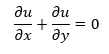
Momentum Equation:

Energy Equation:

The Reynolds-averaged Navier–Stokes equations
The Reynolds-averaged Navier–Stokes equations (RANS equations) are time-averaged equations of motion for fluid flow. The idea behind the equations is Reynolds decomposition, whereby an instantaneous quantity is decomposed into its time-averaged and fluctuating quantities, an idea first proposed by Osborne Reynolds.
The Reynolds-averaged Navier–Stokes equations (RANS equations) are time-averaged equations of motion for fluid flow. The idea behind the equations is Reynolds decomposition, whereby an instantaneous quantity is decomposed into its time-averaged and fluctuating quantities, an idea first proposed by Osborne Reynolds. The RANS equations are primarily used to describe turbulent flows. These equations can be used with approximations based on knowledge of the properties of flow turbulence to give approximate time-averaged solutions to the Navier–Stokes equations. For a stationary flow of an incompressible Newtonian fluid, these equations can be written in Einstein notation in Cartesian coordinates as:

The left hand side of this equation represents the change in mean momentum of a fluid element owing to the unsteadiness in the mean flow and the convection by the mean flow. This change is balanced by the mean body force, the isotropic stress owing to the mean pressure field, the viscous stresses, and apparent stress  owing to the fluctuating velocity field, generally referred to as the Reynolds stress. This nonlinear Reynolds stress term requires additional modeling to close the RANS equation for solving, and has led to the creation of many different turbulence models. The time-average operator is a Reynolds operator.
A mathematical model based on average values of variables for both steady-state and dynamic flows (unsteady for URANS). The numerical simulation is driven by a turbulence model which is arbitrarily selected to find out the effect of turbulence fluctuation on the mean fluid flow.
Derivation of RANS equations
The basic tool required for the derivation of the RANS equations from the instantaneous Navier–Stokes equations is the Reynolds decomposition. Reynolds decomposition refers to separation of the flow variable ( ) into the mean (time-averaged) component (
 ) and the fluctuating component (
 ). Because the mean operator is a Reynolds operator, it has a set of properties. One of these properties is that the mean of the fluctuating quantity is equal to zero
  . Thus,

where  is the position vector. Some authors prefer using
  instead of
  for the mean term (since an overbar is sometimes used to represent a vector). In this case, the fluctuating term is represented instead by . This is possible because the two terms do not appear simultaneously in the same equation. To avoid confusion, the notation , , and will be used to represent the instantaneous, mean, and fluctuating terms, respectively.
The properties of Reynolds operators are useful in the derivation of the RANS equations. Using these properties, the Navier–Stokes equations of motion, expressed in tensor notation, are (for an incompressible Newtonian fluid):


where  is a vector representing external forces.
Next, each instantaneous quantity can be split into time-averaged and fluctuating components, and the resulting equation time-averaged, to yield:


The momentum equation can also be written as,

On further manipulations this yields,

where, 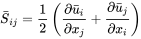 is the mean rate of strain tensor.
Finally, since integration in time removes the time dependence of the resultant terms, the time derivative must be eliminated, leaving:

Equations of Reynolds stress
The time evolution equation of Reynolds stress is given by:

This equation is very complicated. If  is traced, turbulence kinetic energy is obtained. The last term
  is turbulent dissipation rate. All RANS models are based on the above equation.
Applications
A model for testing performance was determined that, when combined with the vortex lattice (VLM) or boundary element method (BEM), RANS was found useful for modelling the flow of water between two contrary rotation propellers, where VLM or BEM are applied to the propellers and RANS is used for the dynamically fluxing inter-propeller state.
Turbulent Viscosity:
Turbulence modeling is the construction and use of a mathematical model to predict the effects of turbulence. Turbulent flows are commonplace in most real life scenarios, including the flow of blood through the cardiovascular system, the airflow over an aircraft wing, the re-entry of space vehicles, besides others. In spite of decades of research, there is no analytical theory to predict the evolution of these turbulent flows. The equations governing turbulent flows can only be solved directly for simple cases of flow. For most real life turbulent flows, CFD simulations use turbulent models to predict the evolution of turbulence. These turbulence models are simplified constitutive equations that predict the statistical evolution of turbulent flows.
The eddy-viscosity based k — є turbulence model has been used in the present work where the additional stresses arising out of turbulent fluctuations in the momentum equations are replaced by viscous type stresses analogous to their laminar counterpart. The turbulent or eddy viscosity μt is defined by the following relationship:
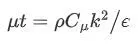
The field distribution of the turbulence kinetic energy k and its dissipation rate є (a measure of turbulence length scale) are obtained from the solution of the relevent transport equations. Since these equations for the turbulence scalars are not strictly valid in the viscosity dominated near wall region, standard Wall Function approach has been used in the present algorithm for the near wall cells.
Turbulence viscosity differ from Molecular viscosity:
The apparent viscosity of a fluid in a turbulent flow is higher than its molecular viscosity. A fluid behaves as a highly viscous fluid when turbulent, hence, requiring extra energy to flow.
The utility of the analogy is strained by the fact that while the molecular viscosity is a property of the fluid, the eddy viscosity is a property of the flow.
The turbulent transfer of momentum by eddies creates internal fluid friction. It is the fundamental idea of how we define viscosity in turbulent flow, i.e. internal fluid resistance. Eddy or turbulence viscosity explains what causes the internal friction.
Molecular viscosity is the same as viscosity. The Coefficient of Molecular Viscosity is the same value as dynamic viscosity.
Molecular viscosity is the transport of mass motion momentum solely by the random motions of individual molecules not moving together in coherent groups. Molecular viscosity is analogous in laminar flow to eddy viscosity in turbulent flow.