Week 4.1 - Genetic Algorithm
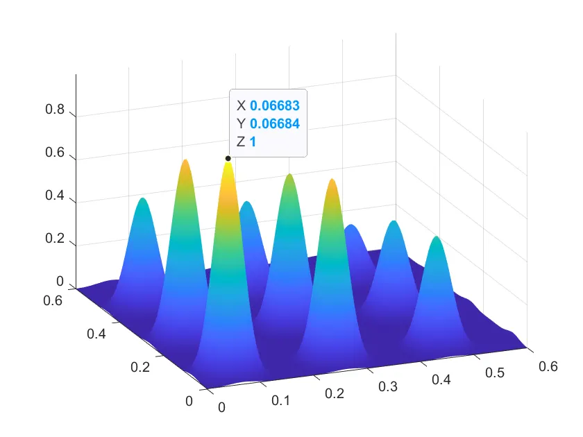
To optimise the stalagmite function and find the global maxima of the function
The genetic algorithm is a technique for solving both constrained and unconstrained optimization problems that are based on natural selection, the process that drives biological evolution.
The genetic algorithm constantly modifies the population size of individual solutions.
% PROVIDING THE SEARCH SPACE FOR THE FUNCTION

    x=linspace(0,0.6,150);
    y=linspace(0,0.6,150);
    [X,Y]=meshgrid(x,y);

    num_cases=50;

% CREATING THE SURFACE PLOT OF STALAGEMITE FUNCTION

     for i=1:length(X)
         for j=1:length(Y)
             input_vector(1)=X(i,j);
             input_vector(2)=Y(i,j);
             f(i,j)=stalagmite(input_vector);
         end
     end

        surfc(X,Y,-f);
        shading interp


% STATISTICAL BEHAVIOUR (UNBOUNDED)

tic
for i=1:num_cases

        [inputs,fopt(i)]=ga(@stalagmite,2);
        xopt(i)=inputs(1);
        yopt(i)=inputs(2);

end
study1_time=toc

        % PLOTING THE GRAPH
        figure(1)

        subplot(2,1,1)

        surfc(X,Y,-f);
        hold on
        shading interp
        plot3(xopt,yopt,-fopt,'marker','o','markersize',5,'markerfacecolor','r');
        xlabel('x');
        ylabel('y');
        grid on
        subplot(2,1,2)
        plot(-fopt);
        xlabel('iterations')
        ylabel('function min value')

% STATISTICAL BEHAVIOUR (BOUNDED)

tic
 for j=1:num_cases

        [inputs,fopt(j)]=ga(@stalagmite,2,[],[],[],[],[0;0],[1;1]);
        xopt(j)=inputs(1);
        yopt(j)=inputs(2);

 end
study2_time=toc

    %PLOTTING
    figure(2)

    subplot(2,1,1)
    hold on
    surfc(X,Y,-f)
    shading interp
    plot3(xopt,yopt,-fopt,'marker','o','markersize',5,'markerfacecolor','r');
    xlabel('x');
    ylabel('y');
    grid on
    subplot(2,1,2)
    plot(-fopt);
    xlabel('iterations')
    ylabel('function min value')

% MODIFYING THE NUMBER OF POPULATION

 options=optimoptions('ga','populationsize',300)


 tic
for k=1:num_cases

    [inputs,fopt(k)]=ga(@stalagmite,2,[],[],[],[],[0;0],[1;1],[],[],options);
     xopt(k)=inputs(1);
     yopt(k)=inputs(2);

end
study3_time=toc

    %PLOTTING
    figure(3)

    subplot(2,1,1)
    hold on
    surfc(X,Y,-f)
    shading interp
    plot3(xopt,yopt,-fopt,'marker','o','markersize',5,'markerfacecolor','r');
    xlabel('x');
    ylabel('y');
    grid on
    subplot(2,1,2)
    plot(-fopt);
    xlabel('iterations')
    ylabel('function min value')
Clearly expalin the concept of genetic algorithm in your own words and also explain the syntax for ga in MATLAB in your report.
Syntax for GA:
[x,fval ,exitflag ,output ,population ,scores]= ga(func,nvars,A,b,Aeq,Beq,lb,ub,nonlcon,Intcon,options)
x = optimum solution
exitflag = reason ga stopped
output= information about optimization process
population=final population
scores= final scores
f=ga(fun,nvars,A,b,[],[],lb,ub,nonlcon,IntCon,options)
fun - fitness function.
nvars- number of variables,
A,b= Linear inequality constraints
Aeq,beq=Linear equality constraints
lb- Lower bound(limit),
ub- Upper bound(limit),
nonlcon : Use for nonlinear constraints
IntCon : to get solution in integer.
options- To set population size minimize with non-default options
BODY OF THE CONTENT:
- FITNESS FNUCTION
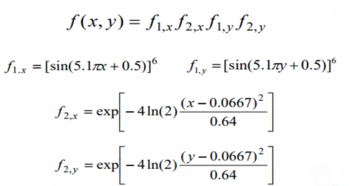
- The above equations are used in the stalagmite function to plot the graph in the main functions.
function [f] = stalagmite(input_vector)

            x = input_vector(1);
            y = input_vector(2);

            f1_x = (sin(5.1*pi*x + 0.5)).^6;
            f1_y = (sin(5.1*pi*y + 0.5)).^6;

            t1 = ((x-0.0667).^2)/(0.64);
            f2_x = exp(-4.*log(2)*t1);

            t2 = ((y-0.0667).^2)/(0.64);
            f2_y = exp(-4.*log(2)*t2);

            f = -(f1_x.*f2_x.*f1_y.*f2_y);

end- While using the function at the end as we are using the -ve sign so that the plot will be reversed as we have to find the maxima of the given function using ga.
- MAIN BODY
- Firstly, creating the mesh from the two vectors which will be acting as a search space to find the maxima of the function.
- Creating the mesh of these two vectors using the ‘mesh’ command and defining the no. of iterations as num_cases to iterate the values of the optimum values of the function.\
- Now calculating the values of fitness function at each point of the mesh grid formed.
- Now creating its surface through ‘surfc’ command which will also provide the contour of the generated surface.
- While using surfc applying the -ve sign to the function will generate the surface upside down which will be quite good to get the maxima of the function, as it will provide positive value for the maxima using the -ve sign.
clear
close all
clc

%% PROVIDING THE SEARCH SPACE FOR THE FUNCTION

    x=linspace(0,0.6,150);
    y=linspace(0,0.6,150);
    [X,Y]=meshgrid(x,y);

    num_cases=50;       %Number of itreation for which the function will evaluate the fitness


%% CREATING THE SURFACE PLOT OF STALAGEMITE FUNCTION

     for i=1:length(X)
         for j=1:length(Y)
             input_vector(1)=X(i,j);
             input_vector(2)=Y(i,j);
             f(i,j)=stalagmite(input_vector);   %values of function in given search space
         end
     end

        surfc(X,Y,-f);       %generating the surface
        shading interp      %To remove the lines produced by the mesh grid
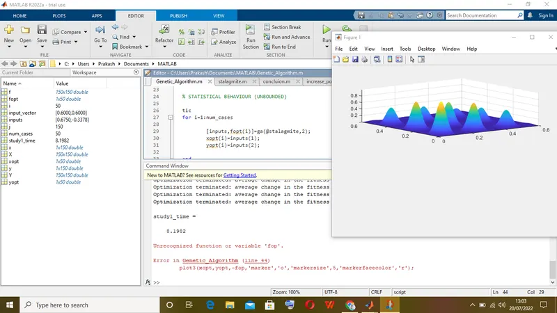
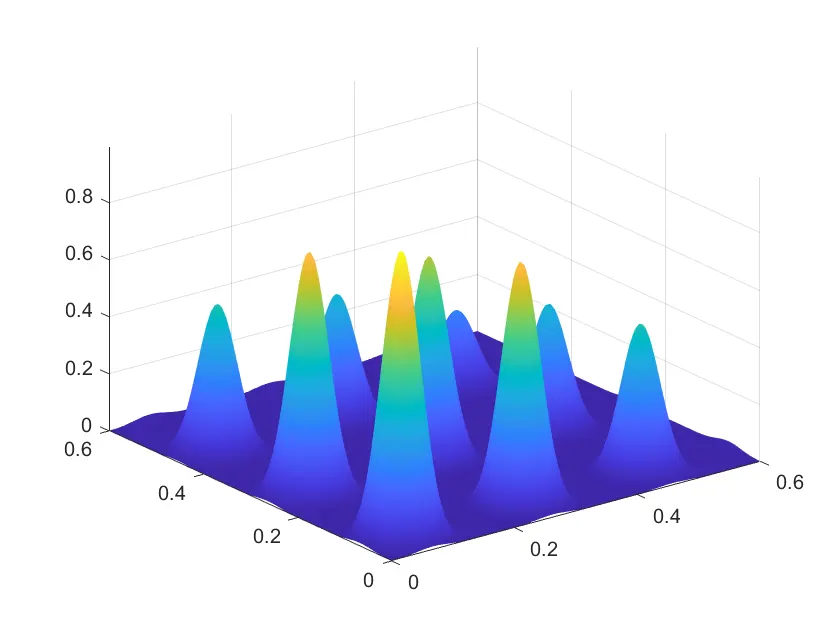
The plot generated is shown below:
- STATISTICAL STUDY WITHOUT BOUNDATION
- In this evaluating the optimum value of fitness function at each iteration and calculating it using the above-mentioned syntax in the intro part (which gives the inputs ie. Values of x and y at which the stalagmite function is minimum)
- Then plotting it into the surf command and also providing the optimum values of the function that how it is varying.
- Also using the tic and tok command to evaluate the time used for optimizing the function.
%% STATISTICAL BEHAVIOUR (UNBOUNDED)

tic                             %calculating the study time through tic and toc command
for i=1:num_cases

        [inputs,fopt(i)]=ga(@stalagmite,2);     %calculating the optimized value of the function
        xopt(i)=inputs(1);                      %at each iteration
        yopt(i)=inputs(2);

end
study1_time=toc                  %displaying the time taken to evaluate

        % PLOTING THE GRAPH
        figure(1)

        subplot(2,1,1)

        surfc(X,Y,-f);
        hold on
        shading interp
        plot3(xopt,yopt,-fopt,'marker','o','markersize',5,'markerfacecolor','r');
        xlabel('x');
        ylabel('y');
        grid on
        subplot(2,1,2)
        plot(-fopt);
        xlabel('iterations')
        ylabel('function min value')
PLOTTING
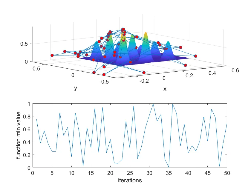
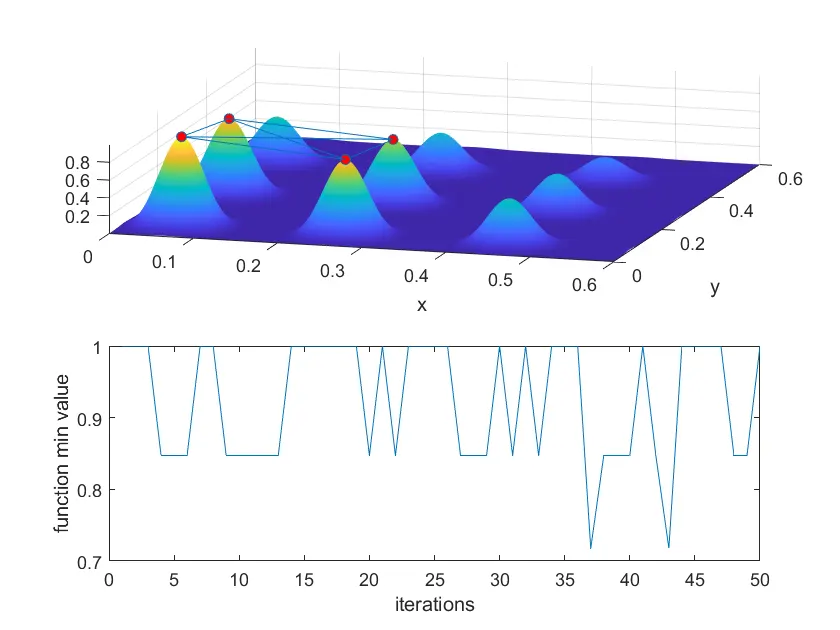
- From the figure as shown above it is clear that the results are not that much accurate and giving a lot of variation in optimizing the function.
STATISTICAL STUDY WITH BOUNDATION
- The difference over here is in providing the upper and the lower limit in the ga so that the search space is reduced with the upper and lower boundary
- And then plotting it as similar to the above study.
%% STATISTICAL BEHAVIOUR (BOUNDED)

tic                                %calculating the study time through tic and toc command
 for j=1:num_cases

        [inputs,fopt(j)]=ga(@stalagmite,2,[],[],[],[],[0;0],[1;1]);   %calculating the optimized value of the function
        xopt(j)=inputs(1);                                            %at each iteration with boundation
        yopt(j)=inputs(2);

 end
study2_time=toc

    %PLOTTING
    figure(2)

    subplot(2,1,1)
    hold on
    surfc(X,Y,-f)
    shading interp
    plot3(xopt,yopt,-fopt,'marker','o','markersize',5,'markerfacecolor','r');
    xlabel('x');
    ylabel('y');
    grid on
    subplot(2,1,2)
    plot(-fopt);
    xlabel('iterations')
    ylabel('function min value')
PLOTTING
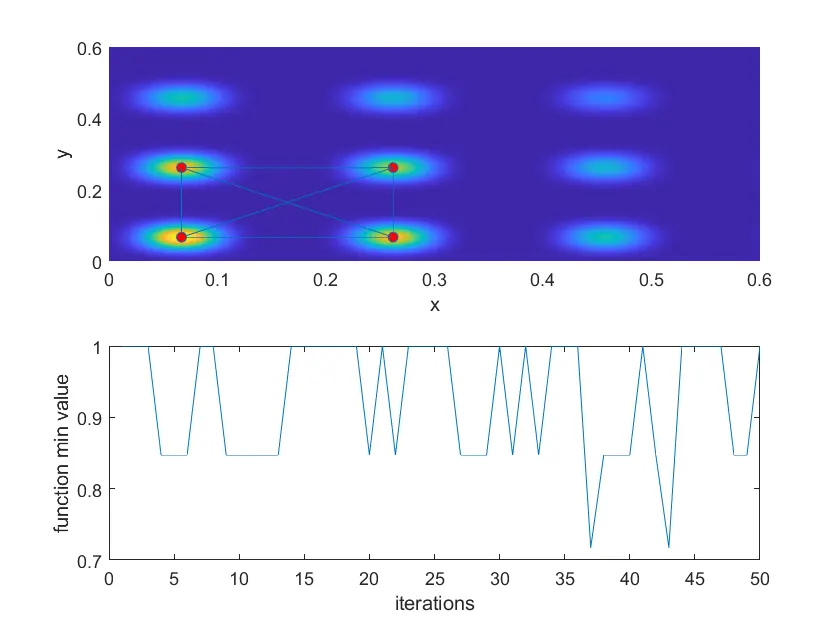
- It is clearly seen from the above that after providing the boundary limits the variation in the optimum value of the function has reduced.
STATISTICAL STUDY WITH INCREASE IN SIZE OF POPULATION
- In this study using the ‘optimoptions’ command to increase the size of population.
- The benefit of that will be it will be working on the large set of numbers and which will be led to increase the possibilities of finding the better fitness of the function.
- The drawback is that the time for evaluation will increase.
options=optimoptions('ga','populationsize',300)        %increaing the sixe of population by using
                                                        %optimoptions function

 tic
for k=1:num_cases

    [inputs,fopt(k)]=ga(@stalagmite,2,[],[],[],[],[0;0],[1;1],[],[],options);
     xopt(k)=inputs(1);
     yopt(k)=inputs(2);

end
study3_time=toc

    %PLOTTING
    figure(3)

    subplot(2,1,1)
    hold on
    surfc(X,Y,-f)
    shading interp
    plot3(xopt,yopt,-fopt,'marker','o','markersize',5,'markerfacecolor','r');
    xlabel('x');
    ylabel('y');
    grid on
    subplot(2,1,2)
    plot(-fopt);
    xlabel('iterations')
    ylabel('function min value')
ploting
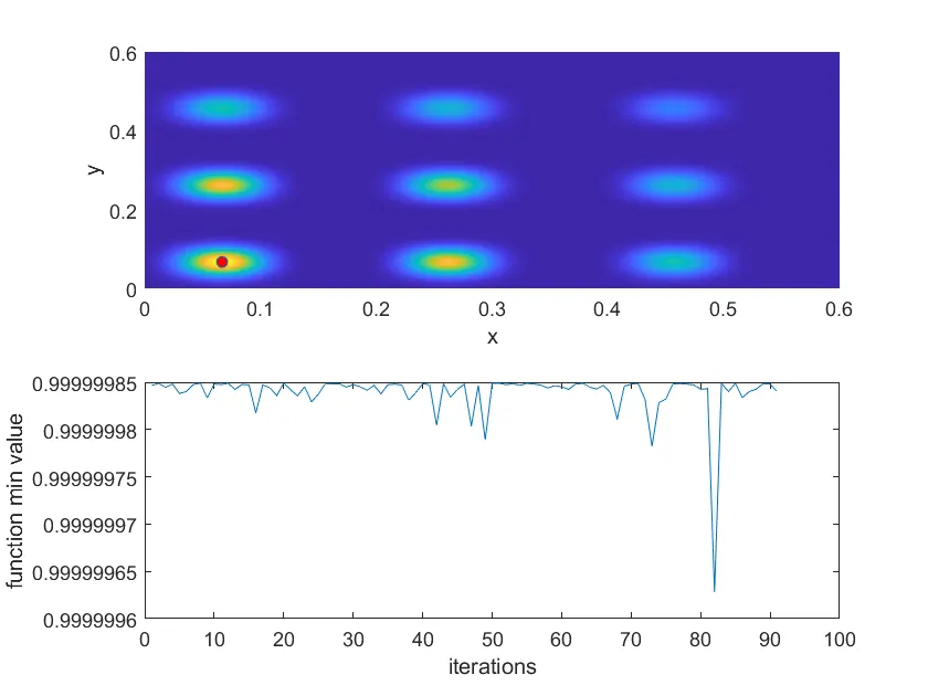
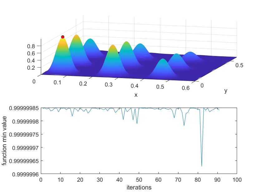
- It is clearly seen in the above case that the value of the variation range has changed to a large extent
ga is useful for optimizing the function but still the result are not accurate as the maximum value for the function lies at -1.
% creating the mesh

x=linspace(0,0.6,150);
y=linspace(0,0.6,150);
 [xx,yy]=meshgrid(x,y);

 % for plotting the surface of stalagmite

 for i=1:length(xx)
     for j=1:length(yy)
         input_vector(1)=xx(i,j);
         input_vector(2)=yy(i,j);
         f(i,j)=stalagmite(input_vector);
     end
 end

 surfc(xx,yy,-f)
 shading interp
% evalutaing the function

    options=optimoptions('ga','PlotFcn',{@gaplotbestf,@gaplotstopping},'populationsize',170);
    [x,fval]=ga(@stalagmite,2,[],[],[],[],[0;0],[1;1],[],options)

        xopt=x(1);
        yopt=x(2);

            figure(1)
            hold on
            plot3(xopt,yopt,-fval,'ro','markersize',5,'markerfacecolor','r')
OUTPUT
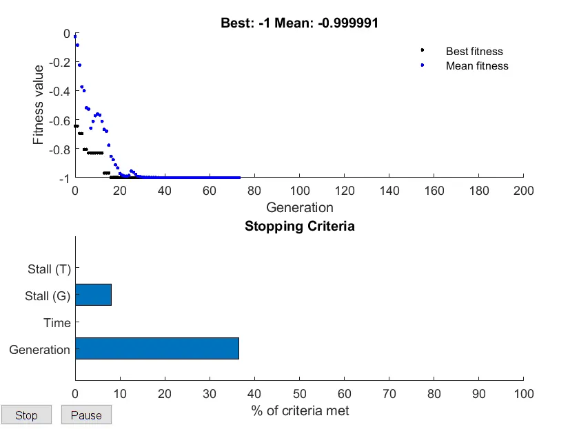
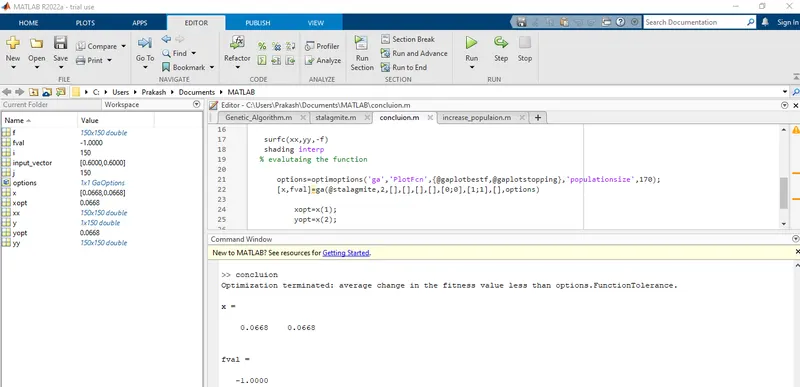
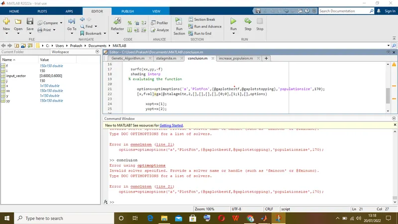
ERROR IN COMMAND WINDOW