Week 7 State of charge estimation
1.Simulate the 3 test cases from harness dashboard and write a detailed report on the results.
Mode-1
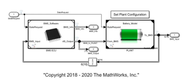
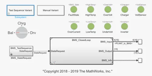
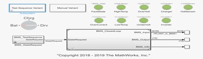
The above fig show the Battery manegament system model.

we set plant configaration Battery 1 pack 1RC
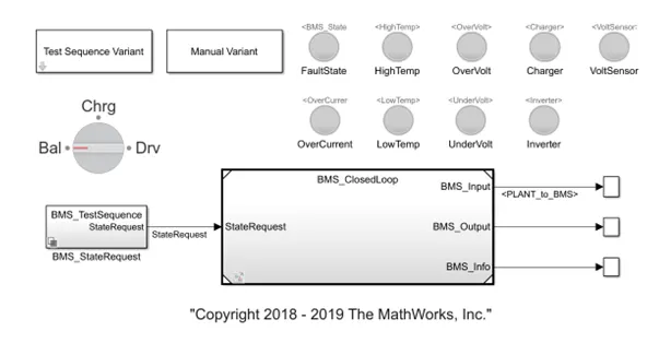
* Click on test sequence variant
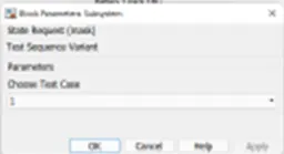
*for mode 01 click 1 in test sequence variant
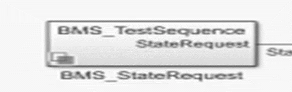
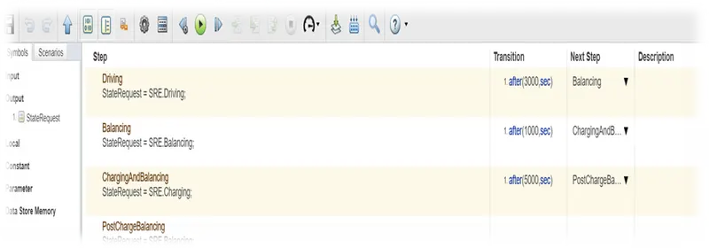
As we look at the test variant as shows above , it states that at the start of the simulation the model will be in the driving condition , thereafter , after 3000 seconds it will be in balancing mode , ofter 1000 seconds it will be in charging and balancing mode and ofter 5000 seconds it will be in post charge balancing mode
results:
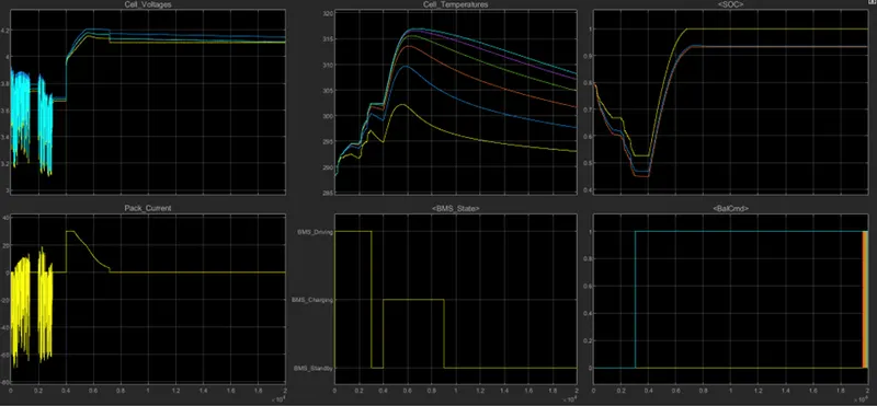
The first plot shows the individual cell voltages , the voltage fluctuates between 3.2 and 3.9 volts between 0 to 3000 seconds . the nominal voltage of each cell is 3.9 volts and it decreases to 3.1 volts
fluctuations in cell voltage from 0 to 3000 seconds shows that the vehicle is in driving mode .
from 3000 to 4000 seconds , we have balancing mode thus cell voltage gets balanced to 4.2 volts till 4000 seconds from 4000 to 6000 seconds , there is charging and balancing stote thus cell voltage rises to 4.1volts
2 ) entire battery pack cument is shown in pack current graph as the curent decreases while charging thus the current is 30A from 0 to 3000 seconds . HEL now from 30001 4000 seconds , there is cell balancing thus pack current reduce to OA O S and from 4000 to 0000 seconds , there is charging state , thus current increases to 30A then occur post charge balancing , thus pack current comes to DA
3 ) the third graph is cell temperature graph temperature reduces and then at start of charging the cell temperature increases in driving stage as vehicle is in driving mode then during baloncing stage , cell the reducing behaviour the temperature increases suddenly then latter at charging ond post charge balancing , the cell temperature shows
4 ) the IMS state graph shows that during 0 to 3000 seconds shows that the vehicle is in driving mode from 3000 to 4000 seconds , we have standby mode from 4000 to 8000 seconds , there is charging state
5 ) The soc graph test that
during driving state , the SOC reduces from 80 % to 45 %
durna balancina state . SOC remains constant at 45 %
during charging stage , the SOC increases to 100 % and then remains constant .
6 ) the cell balancing signal is shown in the balancecommand graph .
Mode-2
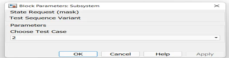
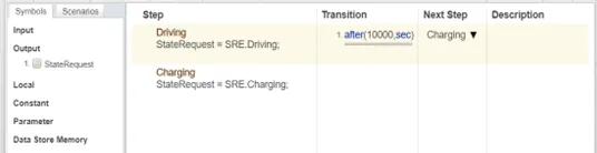
As we look at the test variant as shows above , it states that at the start of the simulation the model will be in the driving condition , thereafter , 0 to 10000 seconds, after 10000 seconds it will be in charging state.
Result:
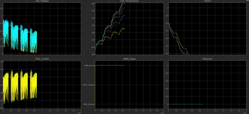
1 ) the cell voltage fluctuates from 3.9 volts to 3.1 volts repeatedly as seen in graph of cell voltages .
2 ) the battery pack current fluctuates from 0 to 20A.
3 ) the cell temperature increases as there is driving stage from 0 to 10000 seconds .
4 ) as driving stage is there from 0 to 10000 sconds , thus BMS graph shows the BMS driving
5 ) the SOC continue to reduce from 80 % to 0 % , the SOC do not increase beacuse there is no charging and balancing stage . though the driving stage is till 10000 seconds but as battery completly discharges at 9000 seconds ( as SOC is 0 % at 9000 seconds ) thus vehicle runs till 9000 seconds only .
Mode:3
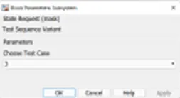

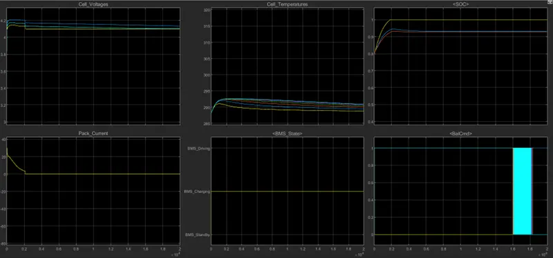
1 ) the cell voltage vories till 20000 seconds and then remians constant
2 ) ot start the pack current increses to 30A and then reduce to 0 A at 2000 seconds and then remains constant at 0A
a ) cells tempearture varies as shown in the graph
3 ) as there is only charging stage
2. What is coulomb counting? Refer to the above model and explain how BMS implements coulomb counting for SOC estimation ?
Coulomb counting
The ‘coulomb counting’ or CoulCount method was developed by Schmitt et al.18 as a heuristic method, although the underlying theory is reasonably accessible.19 It depends on the recording of the current noise only. The signal is filtered with a high-pass filter with a cut-off frequency of 0.01 Hz. The filter may be either analogue (although the implementation of a good-quality 0.01 Hz analogue filter is difficult) or digital. The absolute value of the measured current samples is then summed over time. A steep slope is taken as an indication of rapid corrosion, although it is not possible to calibrate this in terms of an estimated corrosion rate.
It can be shown that this method is similar to integrating the standard deviation of current over time.19 The use of the integrating plot provides a form of low pass filtering that may make it easier to see trends, but this can also be accomplished by digital filtering. The use of only the current noise restricts the value of the technique, as it does not allow for the estimation of the noise resistance (and hence the corrosion rate), and it is difficult to see what real advantages the method has over the conventional threeelectrode method, although the use of integrating plots may be of value.
To determine available capacity, coulomb counting relies on the integration of the current drawn from and supplied to a battery over time, as given by
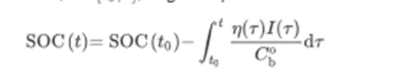
where I is the current and η is the efficiency during charge and discharge operations [4]. Coulomb counting is advantageous in terms of a simple structure and its ease of implementation. However, some problems make it difficult to accurately estimate battery SOC by coulomb counting. Because battery capacity and efficiency are significantly influenced by operating temperature and current direction, these factors should be considered to correct for battery SOC. Sensor accuracy is also important because accumulated errors can lead to a drift in the estimated battery SOC. Furthermore, one of the main problems in coulomb counting is that it is necessary to calibrate the initial battery SOC. In several applications, the initialization involves rest and the initial SOC is estimated based on the voltage inversion method described next.
To improve the Coulomb counting method, a new technique called modified Coulomb counting method is proposed. The modified Coulomb counting method uses the corrected current to improve the accuracy of estimation.
The corrected current is the function of discharging current. There is a quadratic relationship between the corrected current and discharging current of battery. By practice of experimental data, corrected current is calculated by the following form

where , and are constant values obtained from the practice experimental data.
In modified Coulomb counting method, SOC is calculated by the following equation:

The experimental results show that the accuracy of the modified Coulomb counting method is superior to the conventional Coulomb counting method.
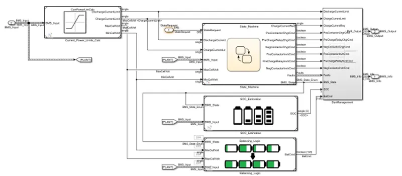
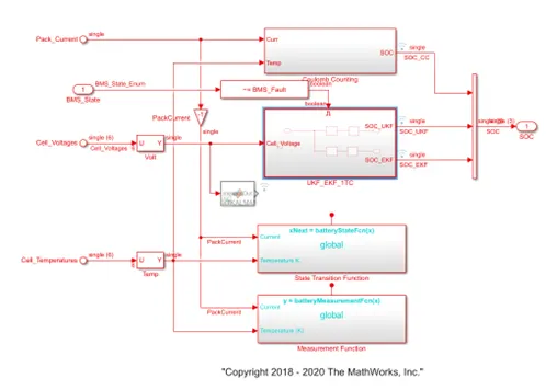
The above fig shows the SOC estimation block
three methods are used for SOC estimation .
there are
1. Coulomb counting method
2. Extended Kalman filter.
3. Unscented Kalman filter.
but coulomb counting is mostly used .
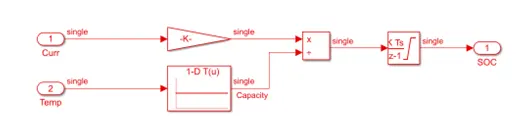
the above fig show the coulomb counting block
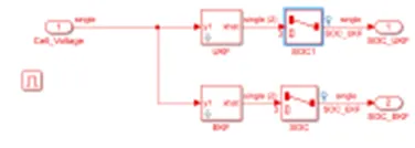
the above fig show the Extended Kalman filter and Unscented Kalman filter
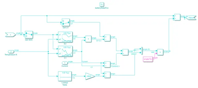
the above fig shows the State Transition Function block
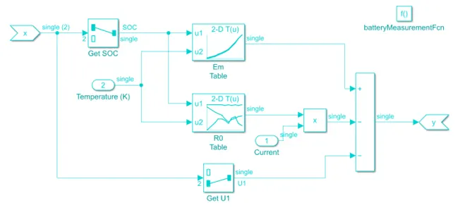
the above fig shows the Measurement Function
1. in this coulomb counting method , the entering and leaving currents of the cell are integrated to track the safe chargable time .
2. here the two input signals current and temperature are taken
3.the curent signal goes to gain block and the temperature signal goes to current look up table .
4.then as seen , signals are multiplied and divided as shown and then output is given to discrete time integrator to track the safe chargable time and then SOC is estimated .
5. advantage of coulomb counting method is its simplicity and low computational cost.
6. the drawback of coulomb counting method is accumulation of current sensor error and inability to recover from wrong initial condition because of lack of feedback from voltage battery