Week 7 State of charge estimation

Objective:-

https://in.mathworks.com/matlabcentral/fileexchange/72865-design-and-test-lithium-ion-battery-management-algorithms

1.Simulate the 3 test cases from harness dashboard and write a detailed report on the results

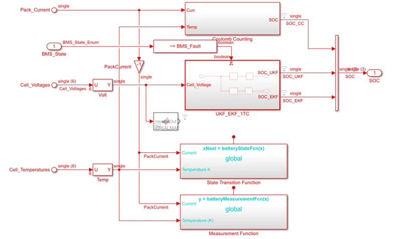
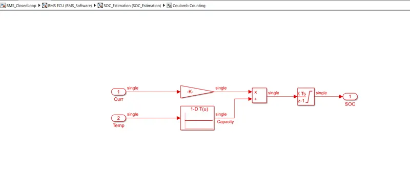
2.What is coulomb counting? Refer to the above model and explain how BMS implements coulomb counting for SOC estimation ?

Result 1:- Simulate the 3 test cases from harness dashboard and write a detailed report on the results.

Test case 1:-

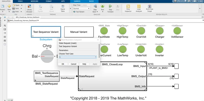
This is the harness dashboard front facia where we will select the objective type to consider and evaluate the result. In the test sequence variant we need to select the test case for result evaluation. For test 1 we have selected 1.

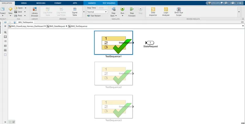
This is the BMS closed loop editor which shows the sequence and timing of driving, discharginf and balancing.

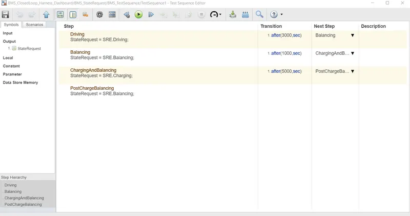
As per the test 1 series we have following sequences:-

• Driving for first 3000 secs
• After 3000 secs balancing procedure will occur for 1000 secs.
• After 1000 secs charging and balancing will occur for 5000 secs.
• After these procedure post charge balancing will occur till the simulation end.

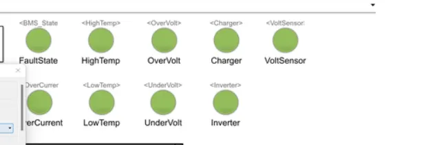
We have run the simulation and waiting for the result for the evaluation. On the dashboard we are seeing some of the indications which shoes the status which shows green for true and red for false or faulty condition. After running program it is showing green it means program is healthy and system is also healthy.

Result of test case 1:-

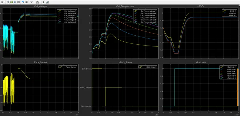
As per the result we have some conclusion-

Cell voltage:- As we know there are 6 nos cell configuration which chracterstics are in the graph. As per the procedure for first 3000 secs cells are in driving mode. Where discharging occurs. During that from 1384 secs to 1880 secs these are in standstill so voltage are in constant mode. In this range voltage value is 3.1 - 3.9V. Constant value of voltage at standstill position is 3.739V. After 3000 secs cell balacninf started which will explain after some time.

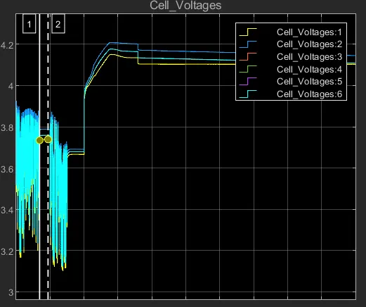
After 4000 secs charging occurs and this charging occurs with constant voltage and constant current mode.

Voltage raised from 3.72V to 4.2V with constant current of 30Amps. After that voltage become constant at 4.2V and current reduces from 2.2Amps.

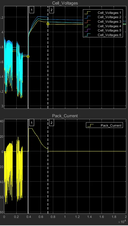
Then charging and balancing occurs upto 9000 secs. After that post charge balacing has been started. Cell balancing will be done as per th cell 1 voltage for making it equivalent.

Peak current:- Explained peak current graph as well in the cell voltage. This is also vary as per the driving till 3000 secs where accelrating and deaccelrating both occurs. current from 20amps- -75amps as per the driving. then again between it standstill condition, then after 3000 secs chargin for 1000 secs. then again charging and balancing occur.

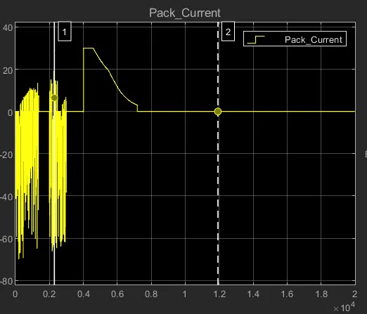
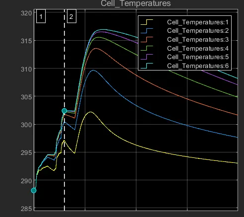
Cell temperature:- Initially during driving till 3000 secs the temperature is gradually increasing. the maximum temp is of cell 6 which is 288K to 302K in this region. between 3000 secs to 4000 secs balancing region so temp are at constant range. after 4000 secs temp start increasing till current constant mode. then decreases till 9000 secs.

BMS State:-

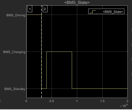
• For 3000 secs battery is in driving mode or call it as discharging mode.
• From 3000-4000 secs for 1000 secs it is in balancing standby mode.
• From 4000-9000 secs for 5000 secs it is in charging and balancing mode.
• After 9000 secs only post charging balancing will occur till simulation end.

SOC:-

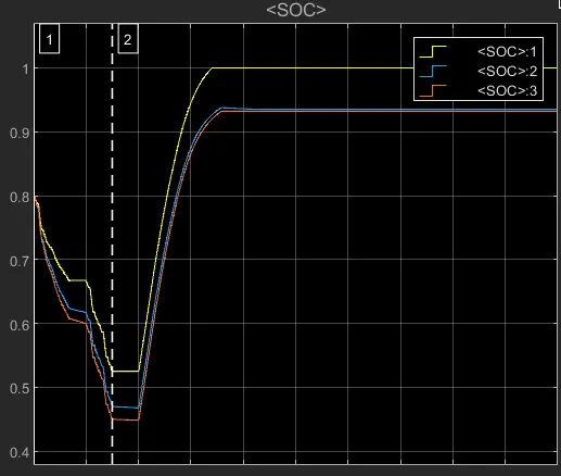
• Initially we can see battery SOC is 80 %. And there are three different colours of battery represents which indicates three different techniques to find SOC.
• Yellow colour plot SOC estimation represents coulomb counting technique.
• Blue colour plot SOC estimation represents unscented kalman filter technique.
• Red colour plot SOC estimation represent Extended kalman filter technique.
• For driving till 3000 secs SOC got decreses till 45% approx.
• After 3000 secs for 1000 secs till 4000 secs it is in constant mode of 45% because of cell balancing occured.
• After 4000-9000 secs it is in charging and balancing mode. from 4000-7000 secs it is in CC mode charging and from 7000-9000 secs it is in CV mode charging.
• After 9000 secs SOC become constant at approx 95%.

Balancing cell:-

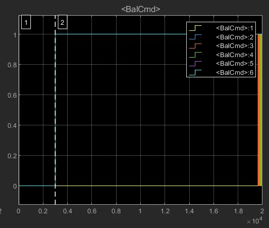
• Till 3000 secs during driving mode no cell balancing occured.
• Between 3000-4000 secs cell balancing occured. And cell 2 and cell 6 rised to 1 as shown in the figure above.
• After 4000-9000 secs its value will be still 1 as shown in the figure till end of the simulation.
• And cell 1 has low voltage which is at 0 state till end of the simulation.
• At the end of the simulation all 6 cells is at equal stage as shown in graph.

Test case 2:-

Now we have selected case 2 as per in the image.

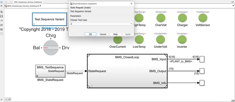
As we can see in the BMS test sequence case 2 has been selected.

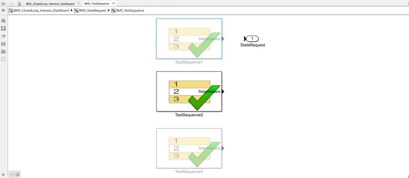
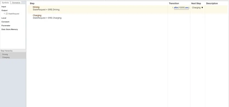
In this test case we have 10000 secs for driving and after that charging occurs till end of the simulation.

Test case 2 Result:- Scope of the result has been showing in the image.

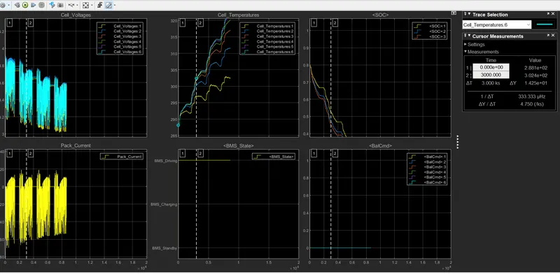
Cell voltage and pack current:-

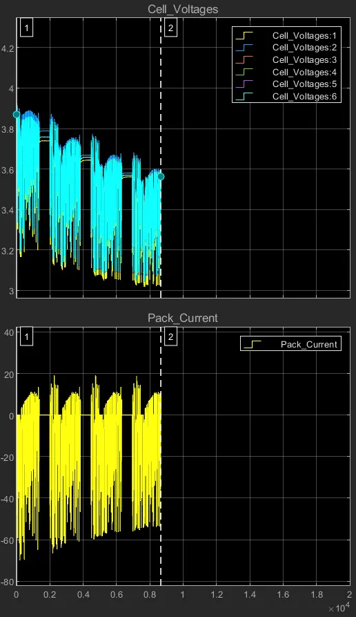
• Cell voltage range from 3.9V- 3.05V approx. The pack current varies from -70Amps - 20Amps. Some negative current also occurs because of Drive cycle which works in regenrative mode.
• both current and voltage works according to drive cycle and works as accelerated and deaccelerated mode. Entire capacity drained at 9000 secs.
• For 10000 secs its driving then charging occured.

Cell temperature:-

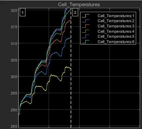
• As per this image cell 1 has least temperature rise and cell 6 has has high temperature rise.
• Cell 1 temp is from 288K to 303K.
• Cell 6 temp is from 288K to 322.5K.
• These cells temperature are increasing decreasing as per the driving and charging period.

BMS:-

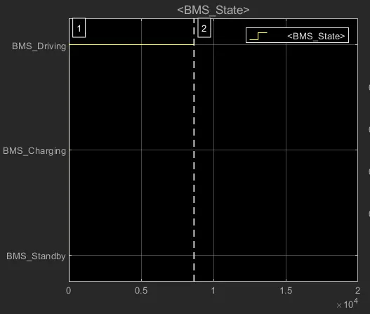
Sequence is running in driving mode as shown in the image.

SOC:-

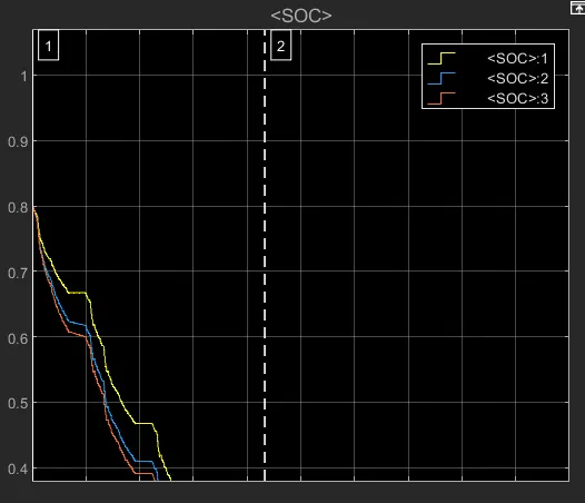
• Initially SOC started from 80%.
• From 80% to 0% during the entire cycle which includes driving and charging.
• During standby mode its value will be constant.

Cell balancing:-

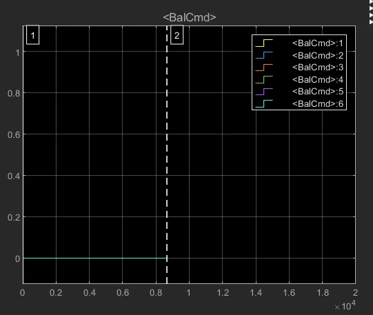
Balancing of cells are not performed in the entire cycle.

Test case 3:-

As here we have done test case 3 which is understood by the image.

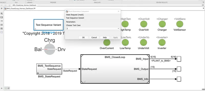
This is the BMS testing sequence which shows which sequence has been selected.

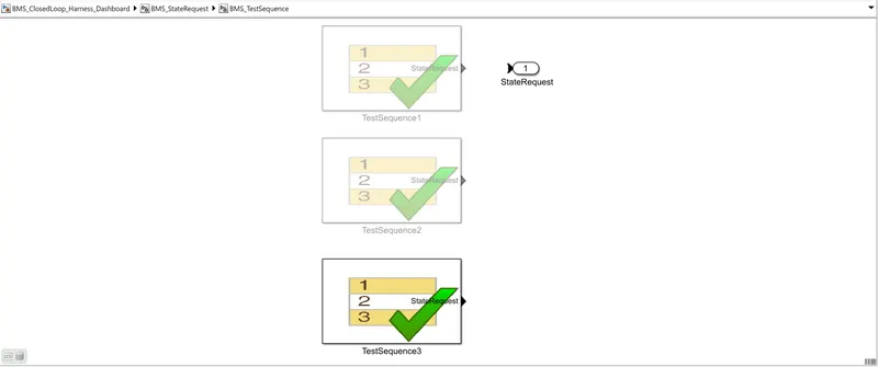
This shows the preocedure that how much operation mentioned as per time limit.

In this test only charging occured.

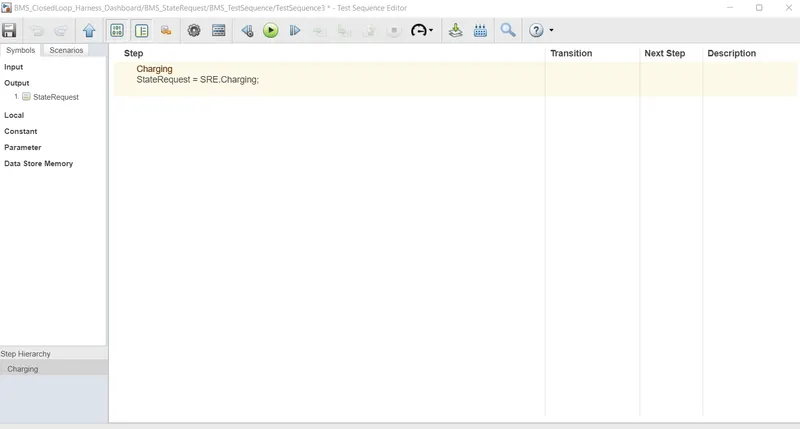
Test case 3 Result:-

We run the simulation and result as as below.

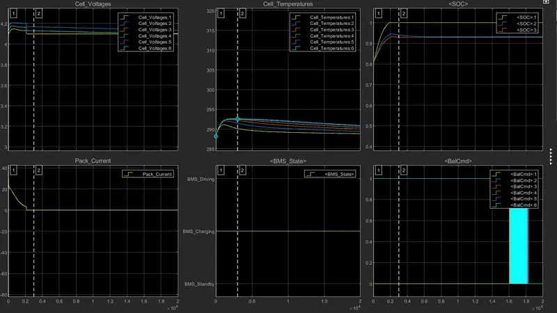
Cell voltage & pack current:-

• By combine we can see the graph of cell voltage and pack current where this case has totally charging state so all cell voltage drasticalaly increase at some point to achieve max voltage.
• By example our cell no 2 voltage is higher from 4.1-4.2V approx then it gets stable at 4.1V.
• All cell voltages getting higher initially at some point then ets stable region.

For the pack current:-

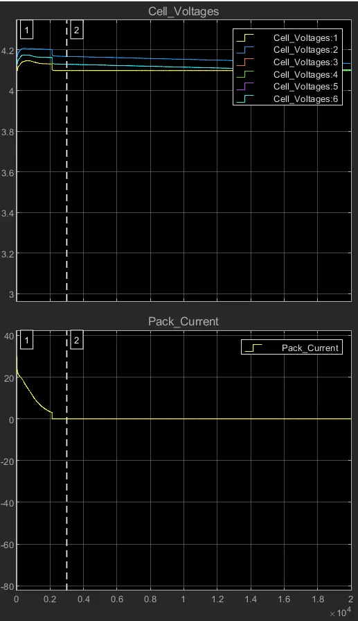
• The battery pack current raising from 0-24Amps approx initially then comes to 2.5Amps approx at the end of 2000 secs of charging state.
• At 2000 secs battery is fully charged.
• At full charging condition current flow will be cut-off.

Cell temperature:-

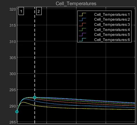
As this is the charing case so initially all cell temperature will be rising and after the period of charging its all getting decreses as shown in the image.

BMS State:-

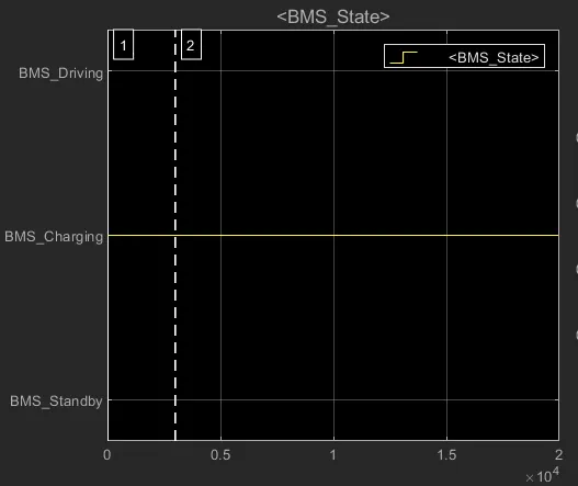
As per this image enitre process is in charging mode as per the BMS.

SOC:-

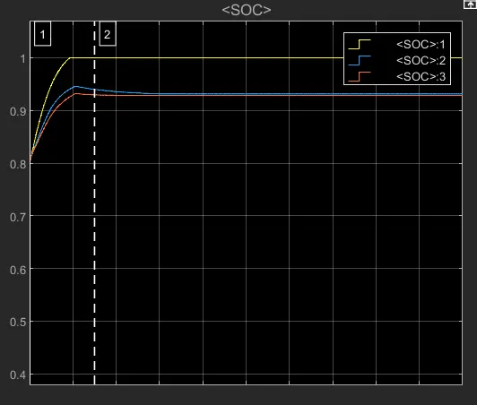
• Again these SOC with three colour plotting shows three different techniques of charging.
• All three techniques getting charged after 2000 secs but the yellow colour shows the coloumb technique which calculate 100% SOC in this image.
• Another two mode which is UKF & EKF SOC is 93% approx which is the true SOC of the cells.

Balancing command:-

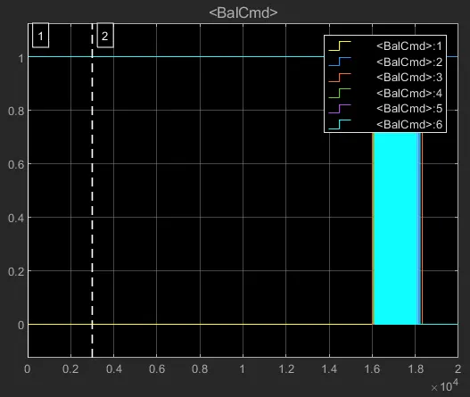
Here again cell 6 and cell 2 starts to balance with respect to cell 1 and all cells trying to balance at the end of the simulation.

Conclusion:-

• Here we have discussed all thee tests of BMS over the model
• Analysed the result with individual parameters.
• We have analysed pack voltage, pack current, cell temperature, BMS, cell balancing and SOC model.

Result 2:- What is coulomb counting? Refer to the above model and explain how BMS implements coulomb counting for SOC estimation ?

Coulomb counting is a technique which is used to track the State of Charge(SOC) of a battery pack. It works by integrating the active flowing current over time to derive the total sum of energy entering or leaving the battery pack. This produces a capacity that is typically measured in Amp-hours.

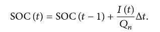
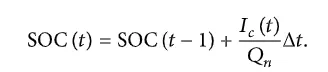
The Coulomb counting method measures the discharging current of a battery and integrates the discharging current over time in order to estimate SOC. Coulomb counting method is done to estimate the , which is estimated from the discharging current, and previously estimated SOC values, SOC is calculated by the following equation:

But there are several factors that affect the accuracy of Coulomb counting method including temperature, battery history, discharge current, and cycle life.

Modified Coulomb counting method:-

To improve the Coulomb counting method, a new technique called modified Coulomb counting method is proposed. The modified Coulomb counting method uses the corrected current to improve the accuracy of estimation.

The corrected current is the function of discharging current. There is a quadratic relationship between the corrected current and discharging current of battery. By practice of experimental data, corrected current is calculated by the following form.

where K2, K1 & K0 and are constant values obtained from the practice experimental data.

In modified Coulomb counting method, SOC is calculated by the following equation

The experimental results show that the accuracy of the modified Coulomb counting method is superior to the conventional Coulomb counting method.

Kalman Filter:-

Using real-time measurement road data to estimate the SOC of battery would normally be difficult or expensive to measure. Application of the Kalman filter method is shown to provide verifiable estimations of SOC for the battery via the real-time state estimation.

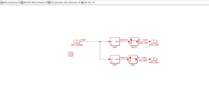
Yatsui and Bai presented a Kalman filter based SOC estimation method for lithium-ion batteries. Experimental results validate the effectiveness of Kalman filter during the online application. Barbarisi et al presented an extended Kalman filter (EKF) to estimate the concentrations of the main chemical species which are averaged on the thickness of the active material in order to obtain the SOC of the battery, by using the terminal current and voltage measurements.

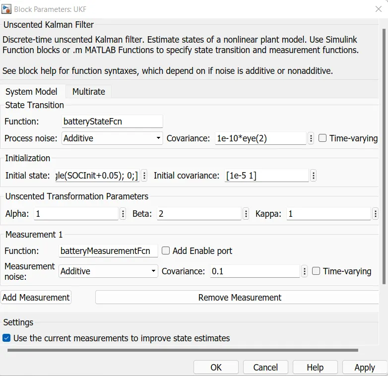
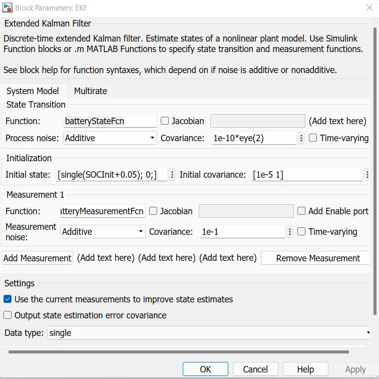
Based on unscented Kalman filter (UKF) theory and a comprehensive battery model, a novel SOC estimation method is proposed in. The results show that UKF method is superior to extended Kalman filter method in SOC estimation for battery. Sun et al. presented an adaptive UKF method to estimate SOC of a lithium-ion battery for battery electric vehicles. The adaptive adjustment of the noise covariance in the SOC estimation process is implemented by an idea of covariance matching in the UKF context.