Week 7 State of charge estimation
3 test cases from the harness dashboard
Matlab model to simulate 3 test cases from harness model was downloaded from the link given below:
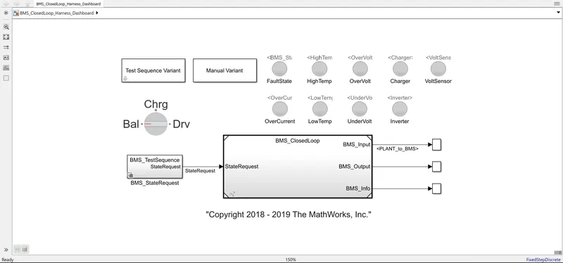
- the test variants can be selected from the test variant block.
- the first test variant is selected for the simulation which is shown below:
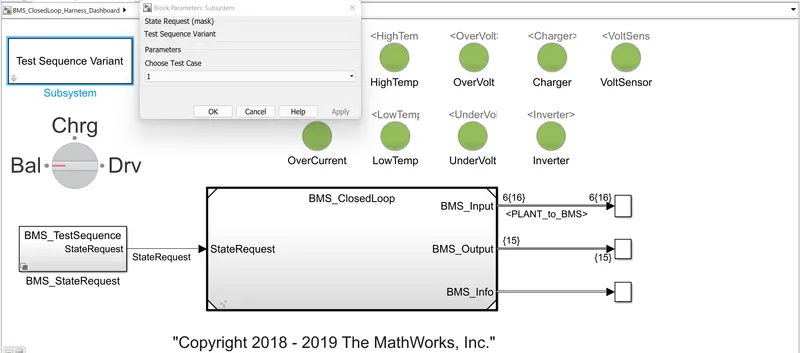
the model is simulated for 20000 seconds. by clicking the bms test sequence block we get the following chart:
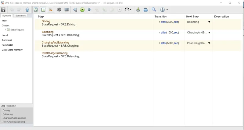
- from the chart it is observed that initially the model will be in driving condition. after 3000 seconds it will enter balancing mode.
- after 1000 sec it will be in charging mode.
- after 5000 sec it will be in post charging balance mode.
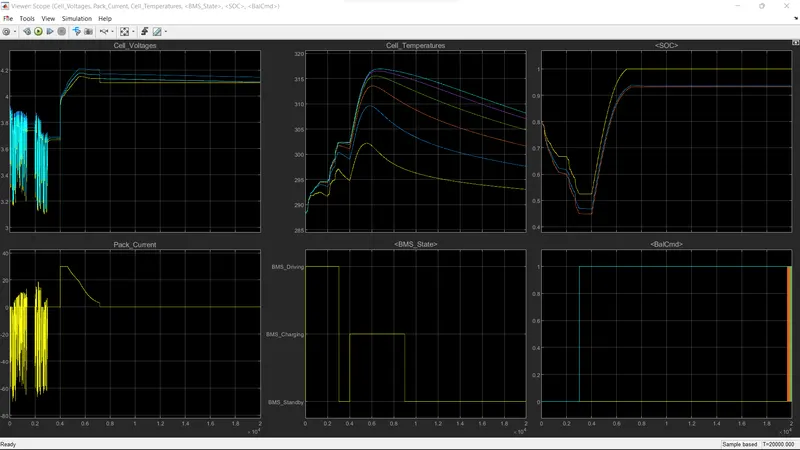
graphs for test variant 1
- from the cell temperature graph, it can be observed that the temperature increases during driving and charging mode.
- it can be observed that the vehicle is in the driving condition in the beginning and charging takes place till 0.98 i.e 98% , continues till it reaches 1 i.e 100%, and reaches standby mode.
- after charging is completed the curve reaches standby mode which is also indicated in BMS state plot as BMS standby.
- the SOC decreased to 45% in driving condition and increased during charging condition and later reached standby mode at 100%.
second test variant
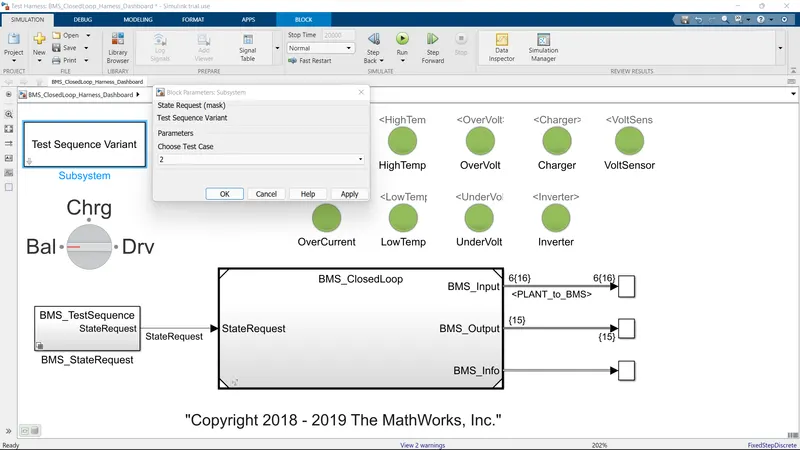
chart
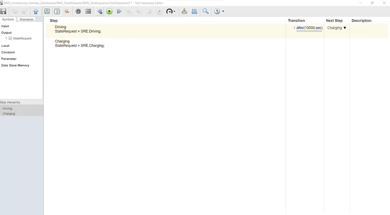
- from the chart, it is observed that initially, the model is in driving condition.
- after 10,000sec it reaches charging condition.
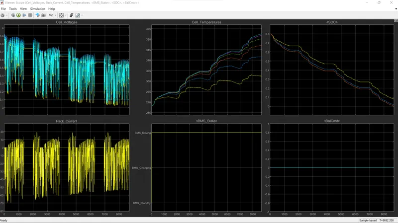
- it is observed that simulation in test 2 variant stops midway as indicated by T=8692 seconds at the bottom right of the graph above.
- the battery gets completely discharged from 80% to 0% as shown in SOC plot.
- there is also a spike in the cell temperature.
- from the BMS state graph, it can be observed that the BMS drive is in standby condition and the vehicle cannot move in this state.
third test condition
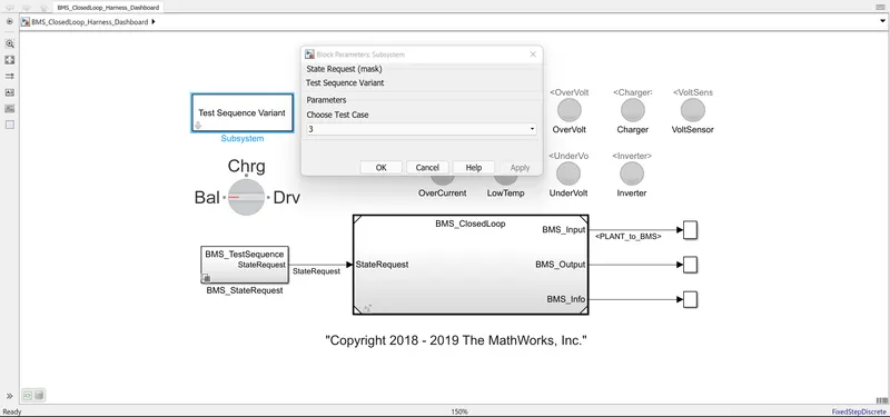
chart
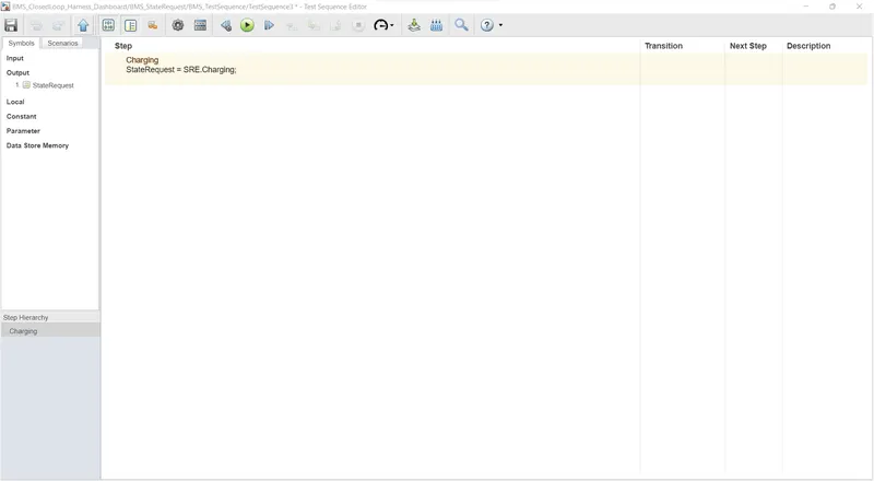
from the chart, it is observed that the model is in continuous charging condition for T=20000 seconds i.e total time for simulation.
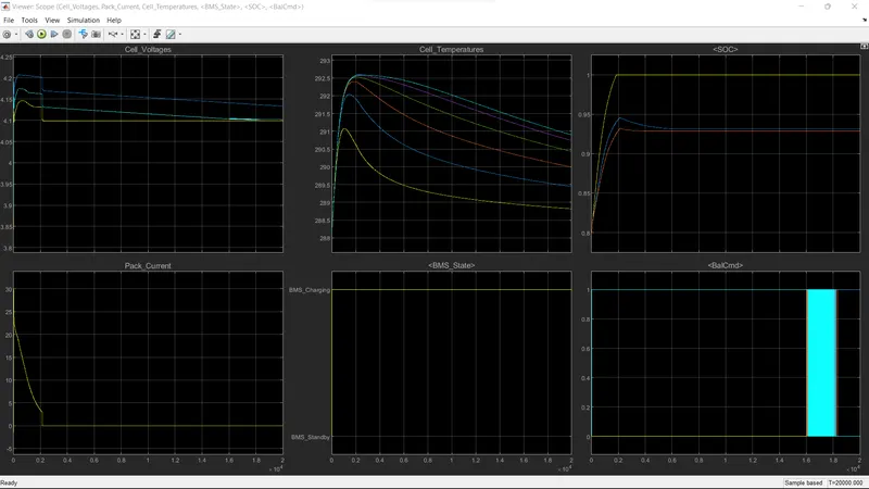
- from the cell temperature plot, it is observed that the temperature increases during charging conditions and gradually reduces during standby conditions.
- battery starts charging and reaches 100% as indicated by the SOC plot.
- the peak current plot drops from 30 to 0 and stays constant as it is continuous charging condition and driving condition is not applied.
2) Columb counting
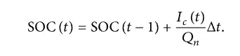
the columb counting method measures the discharging current of battery and integrates the discharging current over time in order to estimate SOC. coloumb counting method is used to estimate the SOC(t), which is estimated from the discharging current I(t) and previously estimated SOC values, SOC(t-1).SOC is calculated by the following equation:
Modified columb counting method
to improve the coloumb counting method a new technique called the Modified Columb counting method is proposed. the modified Columb counting method uses a corrected current to improve the accuracy of the estimation.
the corrected current is the function of discharging current. there is a quadratic relationship between the corrected current and the modified current of the battery. by practice of experimental data corrected current is calculated by the following form

where k2, k1, k0 are constant values.
in modified column counting method SOC is calculated as follows:
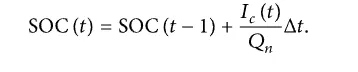
the experimental results show that the accuracy of the modified coloumb counting method is superior to the conventional coloumb counting method.
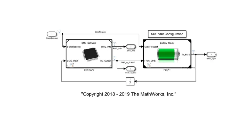
upon selecting BMS ECU block we get
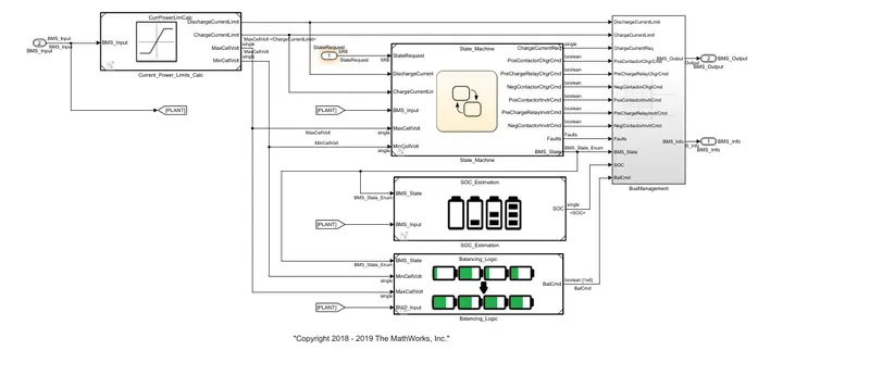
upon clicking SOC estimation block we get:
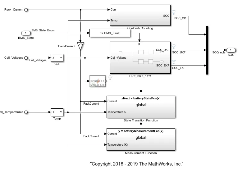
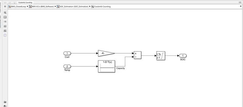
the model of coloumb counting block can be seen below:
- the main advantage of the columb counting method is its simplicity and low computational cost.
- temperature and current are taken as input from the battery.
- the current signal is given to the gain block and temperatures are given to capacity as it varies according to temperature.
- these inputs are given to integration where current will be integrated with respect to time.
- the output is given to another block where it is divided by capacity and SOC is estimated.