Week 7 - Simulation of a 1D Supersonic nozzle flow simulation using Macormack Method
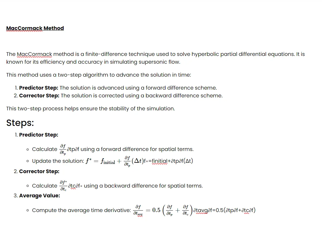
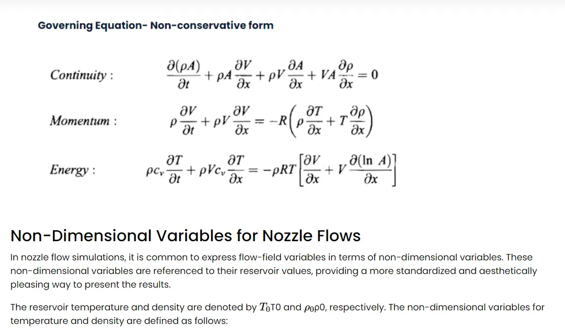
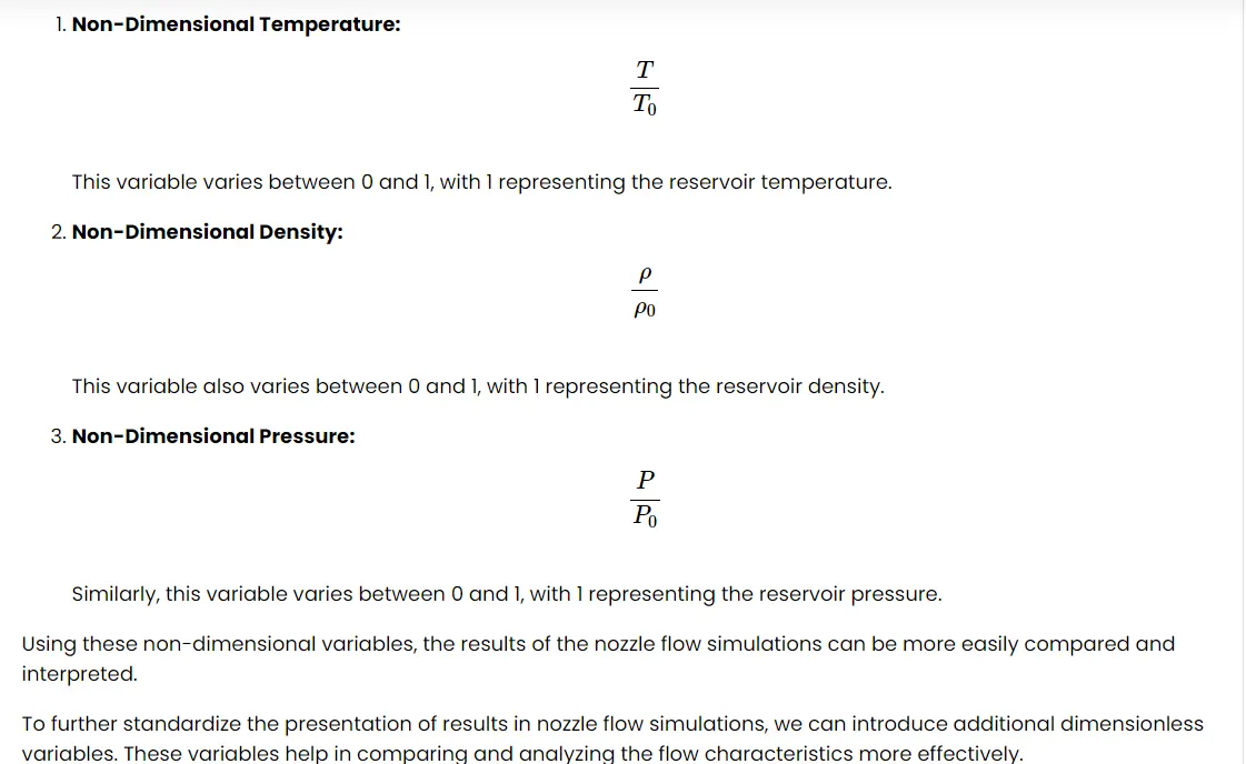
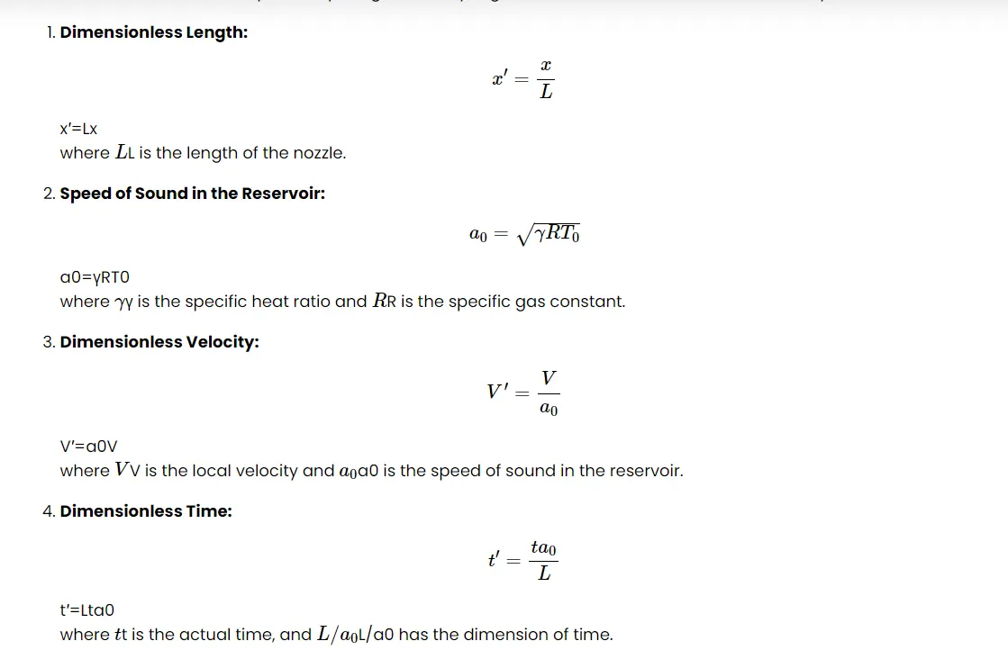
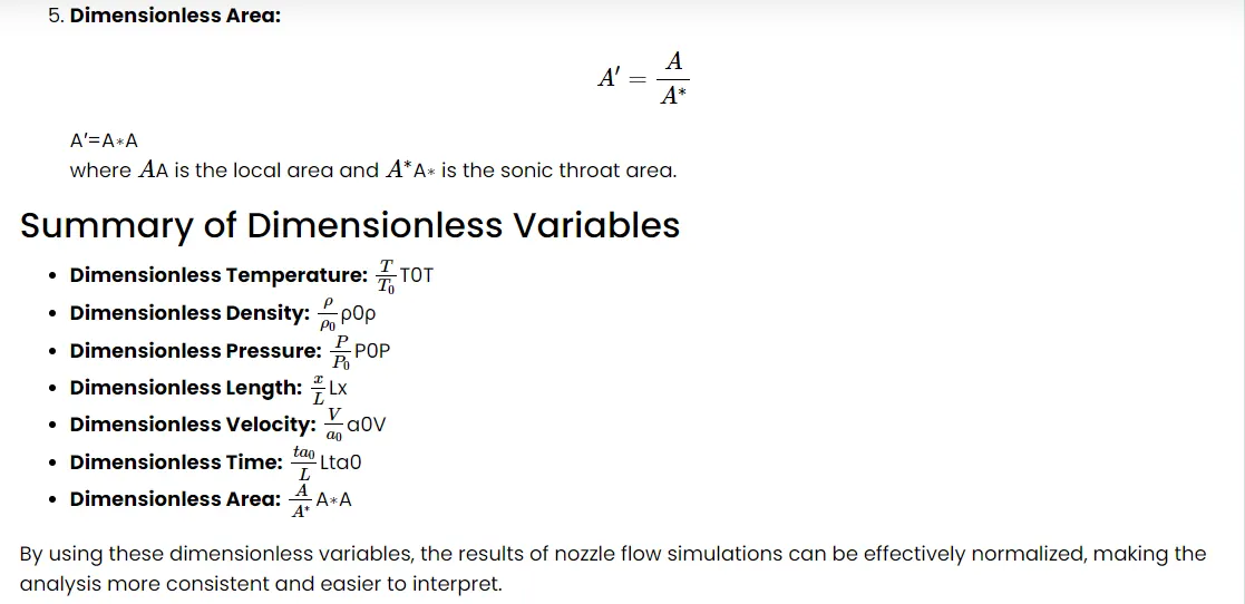
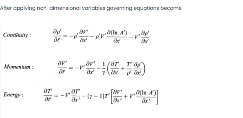
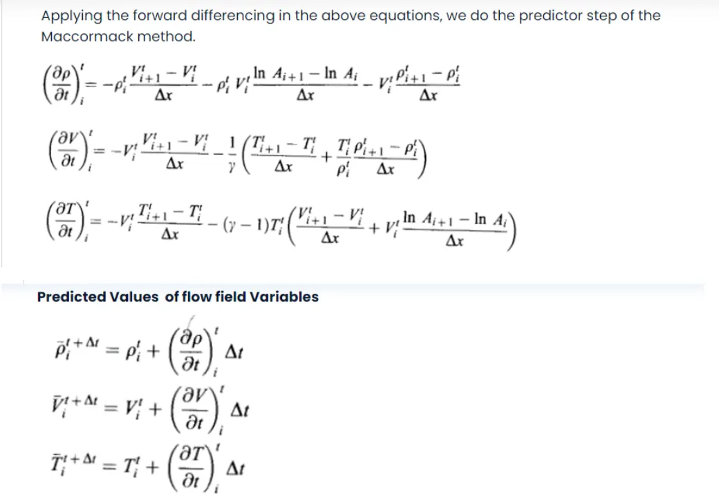
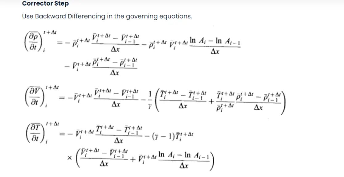
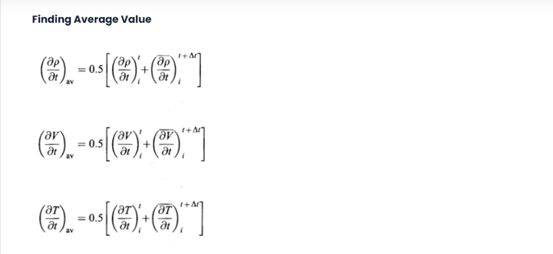
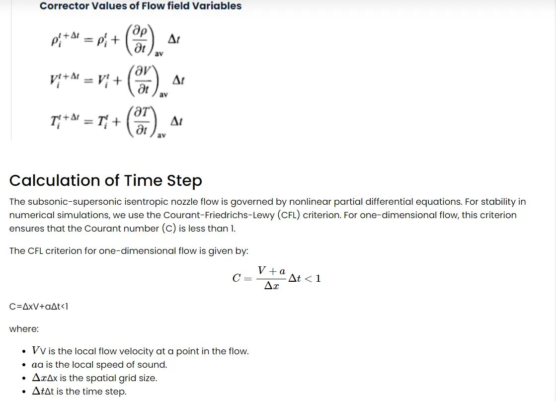
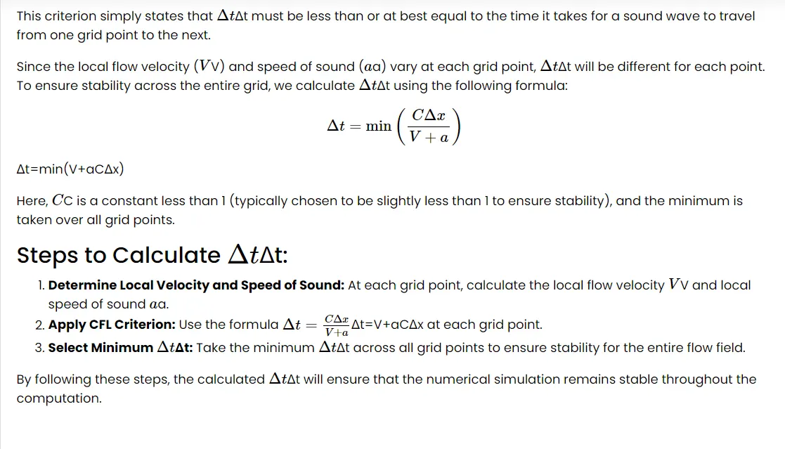
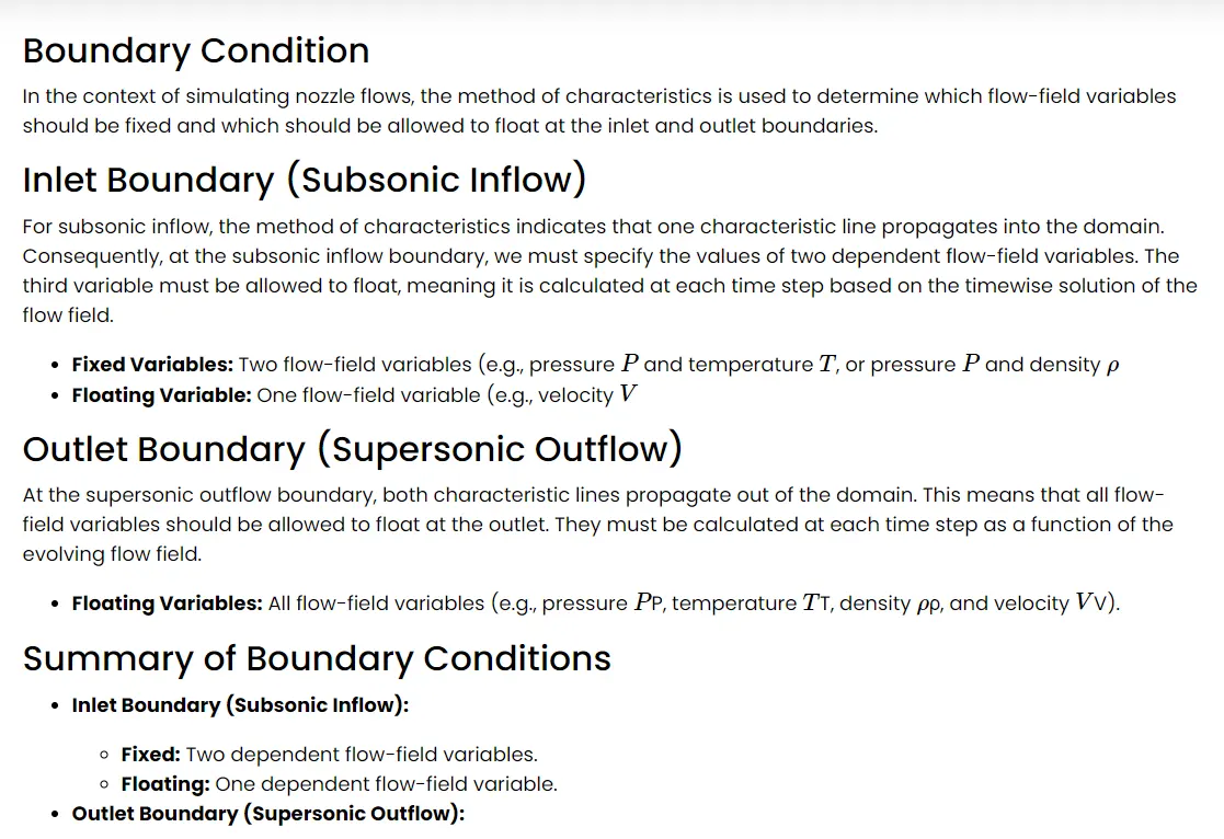
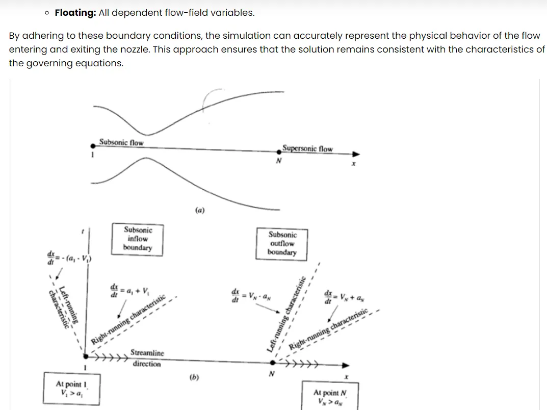
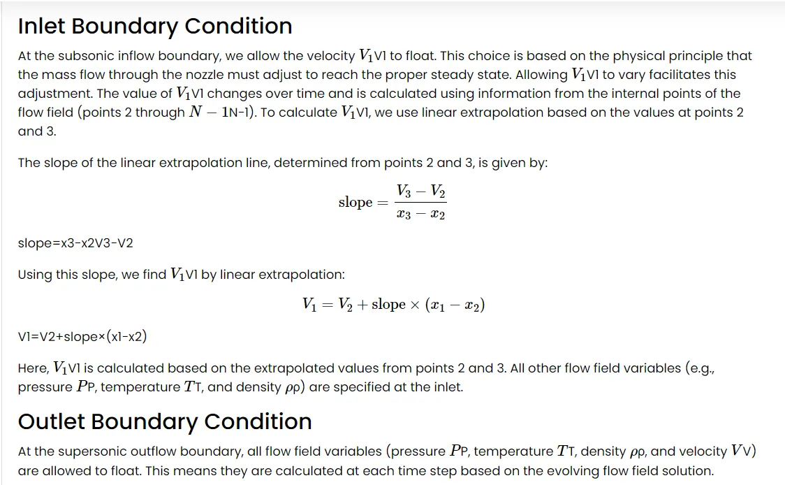
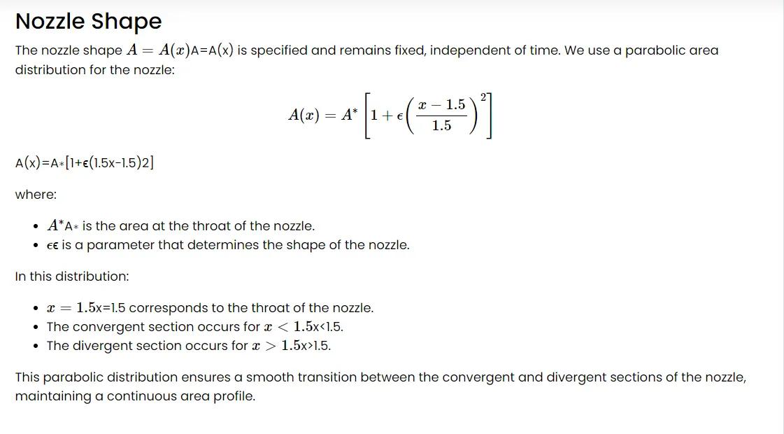
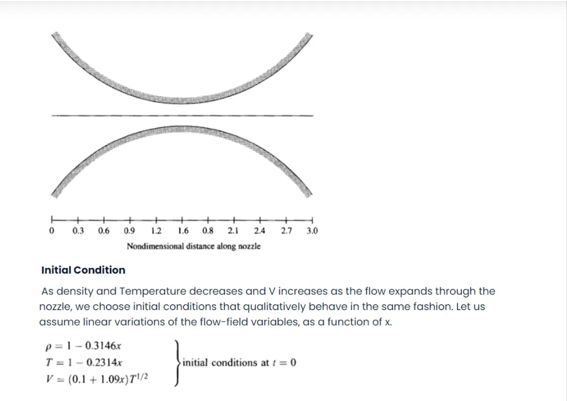
Matlab code for Non-conservative form
% Clear previous data
clear
close all
clc
% Inputs
n = 31; % Number of grid points
x = linspace(0, 3, n); % Discretized spatial domain
dx = x(2) - x(1); % Spatial step size
gamma = 1.4; % Specific heat ratio
% Initial profiles
rho = 1 - 0.3146 * x; % Initial density profile
t = 1 - 0.2314 * x; % Initial temperature profile
v = (0.1 + 1.09 * x) .* t .^ 0.5; % Initial velocity profile
% Nozzle area profile
a = 1 + 2.2 * (x - 1.5) .^ 2;
throat = find(a == 1); % Locate throat position
% Time steps
nt = 1400; % Number of time steps
CFL = 0.5; % CFL number
dt = min((CFL .* dx) ./ (v + sqrt(t))); % Time step size
% Outer time loop
for k = 1:nt
% Store old values for the corrector step
rho_old = rho;
v_old = v;
t_old = t;
% Predictor step
for j = 2:n-1
% Calculate derivatives
dvdx = (v(j+1) - v(j)) / dx;
drhodx = (rho(j+1) - rho(j)) / dx;
dtdx = (t(j+1) - t(j)) / dx;
dlogadx = (log(a(j+1)) - log(a(j))) / dx;
% Continuity equation
drhodt_p(j) = -rho(j) * dvdx - rho(j) * v(j) * dlogadx - v(j) * drhodx;
% Momentum equation
dvdt_p(j) = -v(j) * dvdx - (1 / gamma) * (dtdx + (t(j) / rho(j)) * drhodx);
% Energy equation
dtdt_p(j) = -v(j) * dtdx - (gamma - 1) * t(j) * (dvdx + v(j) * dlogadx);
% Solution update
rho(j) = rho(j) + drhodt_p(j) * dt;
v(j) = v(j) + dvdt_p(j) * dt;
t(j) = t(j) + dtdt_p(j) * dt;
end
% Corrector step
for j = 2:n-1
% Calculate derivatives
dvdx = (v(j) - v(j-1)) / dx;
drhodx = (rho(j) - rho(j-1)) / dx;
dtdx = (t(j) - t(j-1)) / dx;
dlogadx = (log(a(j)) - log(a(j-1))) / dx;
% Continuity equation
drhodt_c(j) = -rho(j) * dvdx - rho(j) * v(j) * dlogadx - v(j) * drhodx;
% Momentum equation
dvdt_c(j) = -v(j) * dvdx - (1 / gamma) * (dtdx + (t(j) / rho(j)) * drhodx);
% Energy equation
dtdt_c(j) = -v(j) * dtdx - (gamma - 1) * t(j) * (dvdx + v(j) * dlogadx);
% Compute the average time derivative
drhodt(j) = 0.5 * (drhodt_p(j) + drhodt_c(j));
dvdt(j) = 0.5 * (dvdt_p(j) + dvdt_c(j));
dtdt(j) = 0.5 * (dtdt_p(j) + dtdt_c(j));
end
% Final solution update
for i = 2:n-1
rho(i) = rho_old(i) + drhodt(i) * dt;
v(i) = v_old(i) + dvdt(i) * dt;
t(i) = t_old(i) + dtdt(i) * dt;
end
% Applying the boundary conditions
% Inlet
v(1) = 2 * v(2) - v(3);
rho(1) = 1;
t(1) = 1;
% Outlet
v(n) = 2 * v(n-1) - v(n-2);
rho(n) = 2 * rho(n-1) - rho(n-2);
t(n) = 2 * t(n-1) - t(n-2);
% Calculating derived quantities
p = rho .* t; % Pressure
mass_flow_rate = rho .* a .* v; % Mass flow rate
mach_no = v ./ sqrt(t); % Mach number
% Storing values at the throat for time-wise plots
p_throat(k) = p(throat);
rho_throat(k) = rho(throat);
v_throat(k) = v(throat);
t_throat(k) = t(throat);
mass_flow_rate_throat(k) = mass_flow_rate(throat);
mach_no_throat(k) = mach_no(throat);
% Storing mass flow rates at specific time steps for comparison
if k == 50
m_50 = mass_flow_rate;
end
if k == 100
m_100 = mass_flow_rate;
end
if k == 150
m_150 = mass_flow_rate;
end
if k == 200
m_200 = mass_flow_rate;
end
if k == 700
m_700 = mass_flow_rate;
end
end
% Plotting the results
% Steady state distribution of primitive variables
figure(1)
subplot(4,1,1)
plot(x, mach_no)
xlabel('Length of the nozzle')
ylabel('Mach No')
title('Steady state distribution of primitive variables (Non-Conservative form)')
subplot(4,1,2)
plot(x, p)
xlabel('Length of the nozzle')
ylabel('Pressure')
subplot(4,1,3)
plot(x, rho)
xlabel('Length of the nozzle')
ylabel('Density')
subplot(4,1,4)
plot(x, t)
xlabel('Length of the nozzle')
ylabel('Temperature')
% Time-wise variation of primitive variables at the throat
figure(2)
subplot(4,1,1)
plot(1:nt, p_throat)
ylabel('Pressure')
title('Time-wise variation of primitive variables (Non-Conservative form)')
subplot(4,1,2)
plot(1:nt, rho_throat)
ylabel('Density')
subplot(4,1,3)
plot(1:nt, t_throat)
ylabel('Temperature')
subplot(4,1,4)
plot(1:nt, mach_no_throat)
ylabel('Mach No')
% Mass flow rate distribution
figure(3)
plot(x, mass_flow_rate)
xlabel('Length of the nozzle')
ylabel('Mass flow rate')
title('Mass flow rate distribution (Non-Conservative form)')
% Mass flow rate at the throat over time
figure(4)
plot(1:nt, mass_flow_rate_throat)
xlabel('Different Time steps')
ylabel('Mass flow rate at throat')
title('Mass flow rate distribution at throat (Non-Conservative form)')
% Comparison of mass flow rates at different time steps
figure(5)
plot(x, m_50, 'r')
hold on
plot(x, m_100, 'b')
hold on
plot(x, m_150, 'y')
hold on
plot(x, m_200, 'm')
hold on
plot(x, m_700, 'g')
title('Mass flow rates at different Timesteps - Conservative form')
xlabel('Length of the nozzle')
ylabel('Mass flow rate')
legend({'50th Timestep', '100th Timestep', '150th Timestep', '200th Timestep', '700th Timestep'})
grid on
This script follows these steps:
- Initializes the spatial grid and flow variables.
- Sets up the nozzle area profile.
- Determines the time step size based on the CFL condition.
- Performs the time-marching process using the MacCormack method with predictor and corrector steps.
- Applies boundary conditions at each time step.
- Plots the results, including the steady-state distribution of primitive variables, time-wise variation of variables at the throat, mass flow rate distribution, and comparison of mass flow rates at different time steps.
The code includes detailed comments to help understand each section and the purpose of each calculation.
Initial Conditions
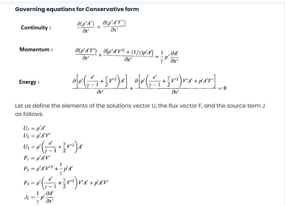
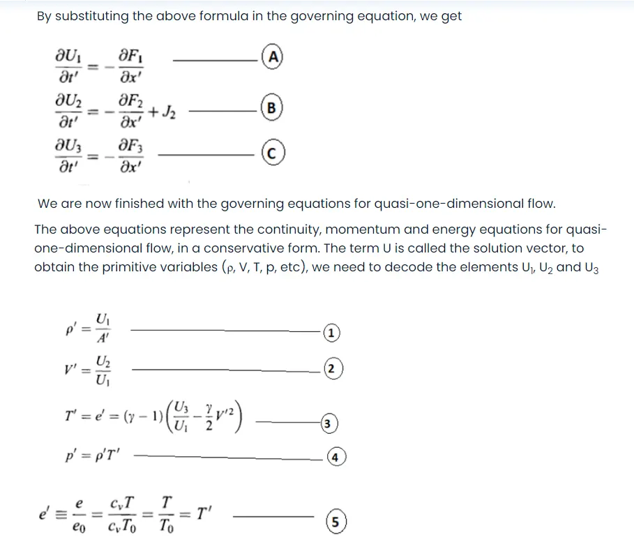
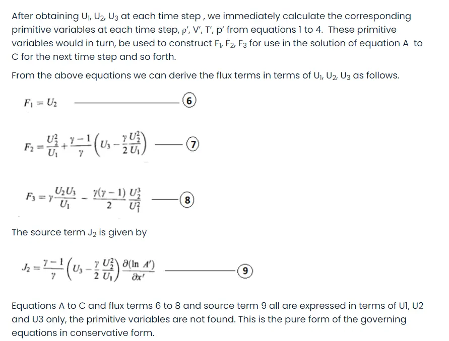
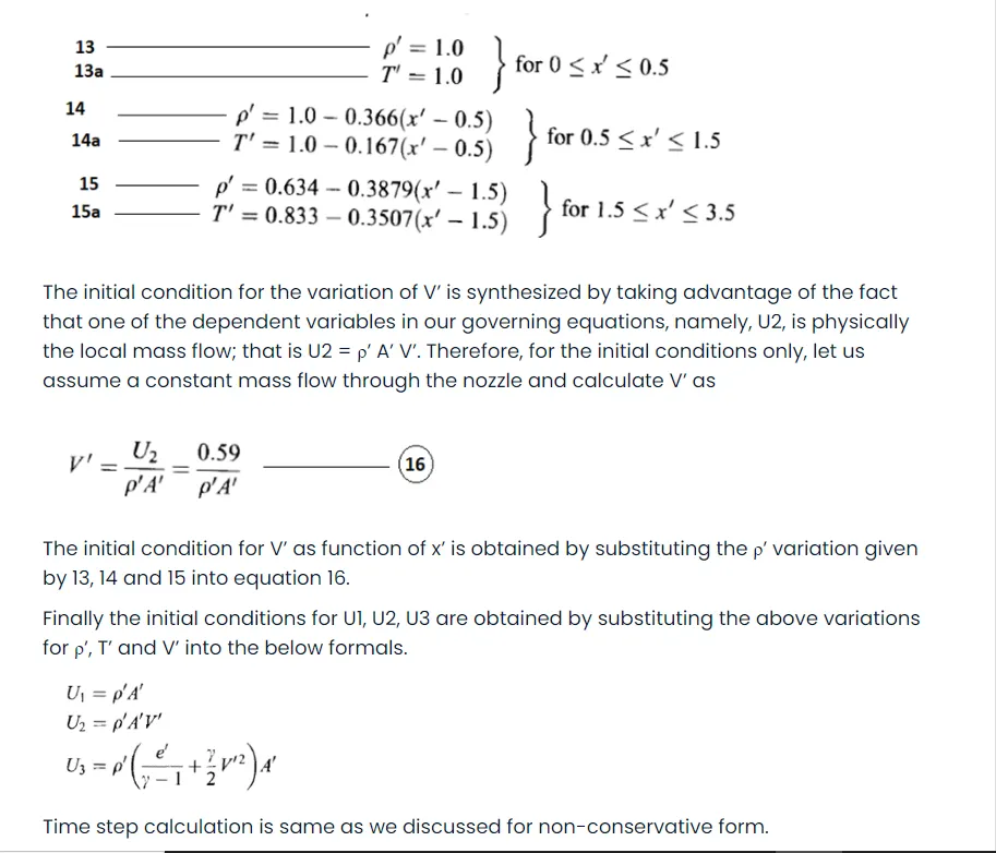
The initial conditions for U1, U2 and U3 were calculated by assuming the following variations of ρ’ and T’
Matlab code for Conservative form of Quasi-one-dimensional flow
% Clear all previous data and close all figures
clear all
close all
clc
% Define constants and initial setup
n = 31; % Number of grid points
x = linspace(0, 3, n); % Create grid from 0 to 3
dx = x(2) - x(1); % Calculate grid spacing
gamma = 1.4; % Specific heat ratio
% Calculate initial density (rho) and temperature (t) profiles
for i = 1:length(x)
if x(i) < 0.5
rho(i) = 1;
t(i) = 1;
elseif x(i) < 1.5
rho(i) = 1 - 0.366 * (x(i) - 0.5);
t(i) = 1 - 0.167 * (x(i) - 0.5);
else
rho(i) = 0.634 - 0.3879 * (x(i) - 1.5);
t(i) = 0.833 - 0.3507 * (x(i) - 1.5);
end
A(i) = 1 + 2.2 * (x(i) - 1.5)^2; % Area profile
end
throat = find(A == 1); % Locate the throat (minimum area)
p = rho .* t; % Initial pressure
v = 0.59 ./ (rho .* A); % Initial velocity
U1 = rho .* A;
U2 = rho .* A .* v;
U3 = rho .* ((t / (gamma - 1)) + ((gamma / 2) * v.^2)) .* A;
% Set the Courant–Friedrichs–Lewy (CFL) condition
CFL = 0.5;
dt = min((CFL * dx) ./ (v + sqrt(t))); % Time step size
% Time-stepping loop
for k = 1:1400
% Store old values
U1_old = U1;
U2_old = U2;
U3_old = U3;
% Calculate fluxes
F1 = U2;
F2 = (U2.^2 ./ U1) + ((gamma - 1) / gamma) * (U3 - (gamma / 2) * (U2.^2 ./ U1));
F3 = (gamma * U2 .* U3 ./ U1) - (gamma * (gamma - 1) * U2.^3 ./ (2 * U1.^2));
% Predictor step
for i = 2:n-1
J2_p(i) = (1 / gamma) * rho(i) * t(i) * ((A(i + 1) - A(i)) / dx);
dU1dt_p(i) = -(F1(i + 1) - F1(i)) / dx;
dU2dt_p(i) = -(F2(i + 1) - F2(i)) / dx + J2_p(i);
dU3dt_p(i) = -(F3(i + 1) - F3(i)) / dx;
% Update solution
U1(i) = U1(i) + dU1dt_p(i) * dt;
U2(i) = U2(i) + dU2dt_p(i) * dt;
U3(i) = U3(i) + dU3dt_p(i) * dt;
end
% Update primitive variables
rho = U1 ./ A;
v = U2 ./ U1;
t = (gamma - 1) * ((U3 ./ U1) - (gamma / 2) * (v.^2));
% Recalculate fluxes
F1 = U2;
F2 = (U2.^2 ./ U1) + ((gamma - 1) / gamma) * (U3 - (gamma / 2) * (U2.^2 ./ U1));
F3 = (gamma * U2 .* U3 ./ U1) - (gamma * (gamma - 1) * U2.^3 ./ (2 * U1.^2));
% Corrector step
for i = 2:n-1
J2_c(i) = (1 / gamma) * rho(i) * t(i) * ((A(i) - A(i - 1)) / dx);
dU1dt_c(i) = -(F1(i) - F1(i - 1)) / dx;
dU2dt_c(i) = -(F2(i) - F2(i - 1)) / dx + J2_c(i);
dU3dt_c(i) = -(F3(i) - F3(i - 1)) / dx;
end
% Average the rates of change
dU1_dt = 0.5 * (dU1dt_p + dU1dt_c);
dU2_dt = 0.5 * (dU2dt_p + dU2dt_c);
dU3_dt = 0.5 * (dU3dt_p + dU3dt_c);
% Final update
for j = 2:n-1
U1(j) = U1_old(j) + dU1_dt(j) * dt;
U2(j) = U2_old(j) + dU2_dt(j) * dt;
U3(j) = U3_old(j) + dU3_dt(j) * dt;
end
% Update boundary conditions
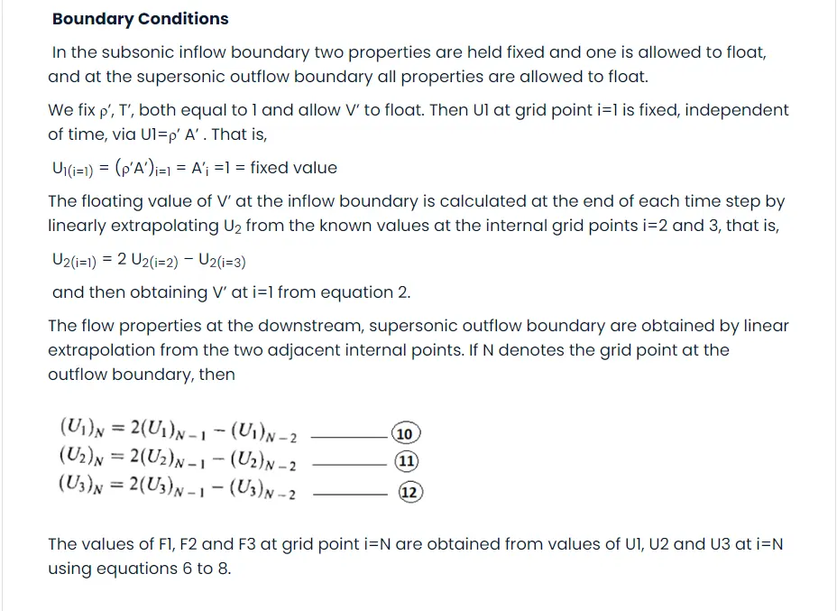
U1(1) = A(1) * rho(1);
U2(1) = 2 * U2(2) - U2(3);
U3(1) = U1(1) * ((t(1) / (gamma - 1)) + (gamma / 2) * v(1)^2);
U1(n) = 2 * U1(n - 1) - U1(n - 2);
U2(n) = 2 * U2(n - 1) - U2(n - 2);
U3(n) = 2 * U3(n - 1) - U3(n - 2);
% Update primitive variables again
rho = U1 ./ A;
v = U2 ./ U1;
t = (gamma - 1) * ((U3 ./ U1) - (gamma / 2) * (v.^2));
p = rho .* t;
mass_flow_rate = rho .* A .* v;
mach_no = v ./ sqrt(t);
% Store throat values at each time step
rho_throat(k) = rho(throat);
v_throat(k) = v(throat);
t_throat(k) = t(throat);
mass_flow_rate_throat(k) = mass_flow_rate(throat);
mach_no_throat(k) = mach_no(throat);
% Save mass flow rate at specific time steps
if k == 50, m_50 = mass_flow_rate; end
if k == 100, m_100 = mass_flow_rate; end
if k == 200, m_200 = mass_flow_rate; end
if k == 700, m_700 = mass_flow_rate; end
if k == 800, m_800 = mass_flow_rate; end
if k == 1000, m_1000 = mass_flow_rate; end
if k == 1400, m_1400 = mass_flow_rate; end
end
% Plot the results
figure(1)
subplot(4, 1, 1)
plot(x, mach_no)
xlabel('Length of the nozzle')
ylabel('Mach No')
title('Steady state distribution of primitive variables (Conservative form)')
subplot(4, 1, 2)
plot(x, p)
xlabel('Length of the nozzle')
ylabel('Pressure')
subplot(4, 1, 3)
plot(x, rho)
xlabel('Length of the nozzle')
ylabel('Density')
subplot(4, 1, 4)
plot(x, t)
xlabel('Length of the nozzle')
ylabel('Temperature')
% Plot time-wise variation of primitive variables at the throat
figure(2)
subplot(3, 1, 1)
plot(1:1400, v_throat)
ylabel('Velocity')
title('Time-wise variation of primitive variables (Conservative form)')
subplot(3, 1, 2)
plot(1:1400, rho_throat)
ylabel('Density')
subplot(3, 1, 3)
plot(1:1400, t_throat)
ylabel('Temperature')
% Plot mass flow rate distribution along the nozzle at the last time step
figure(3)
plot(x, m_1400)
xlabel('Length of the nozzle')
ylabel('Mass flow rate')
title('Mass flow rate distribution through length of the nozzle (Conservative form)')
% Plot mass flow rate at the throat over time
figure(4)
plot(1:1400, mass_flow_rate_throat)
xlabel('Different Time step')
ylabel('Mass flow rate at throat')
title('Mass flow rate distribution (Conservative form)')
% Plot mass flow rates at different time steps
figure(5)
plot(x, m_50)
hold on
plot(x, m_100)
plot(x, m_200)
plot(x, m_700)
plot(x, m_800)
plot(x, m_1000)
plot(x, m_1400)
xlabel('Length of the nozzle')
ylabel('Mass flow rate')
title('Mass flow rate at different time steps')
legend('50', '100', '200', '700', '800', '1000', '1400')
hold off
Output Interpretation:
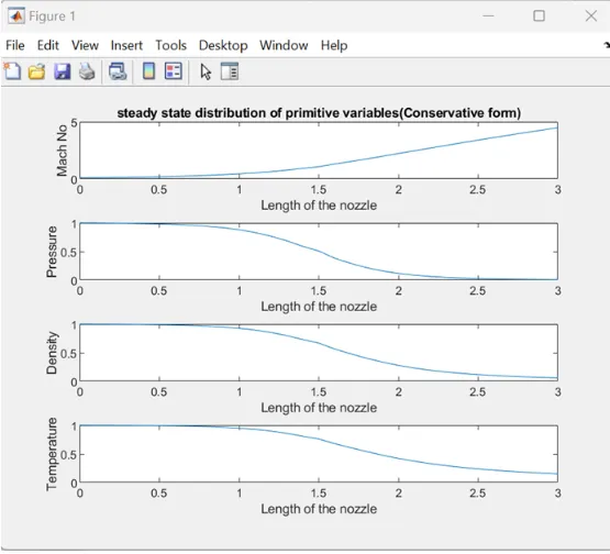
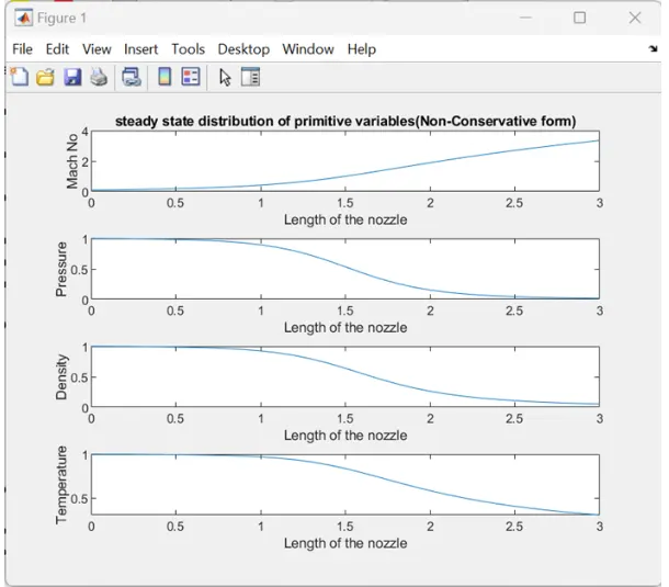
Mach Number Distribution (Figure 1, subplot 1)This plot shows the Mach number along the length of the nozzle.
- The Mach number is subsonic (less than 1) at the inlet.
- The Mach number is supersonic (greater than 1) at the outlet.
- Mach number equals 1 at the throat (length 1.5), indicating that the flow is sonic at this point.
Pressure, Density, and Temperature Distributions (Figure 1, subplots 2-4):
- These plots show how pressure, density, and temperature vary along the length of the nozzle.
- The pressure, density, and temperature profiles adjust as the flow accelerates from subsonic to supersonic speeds.
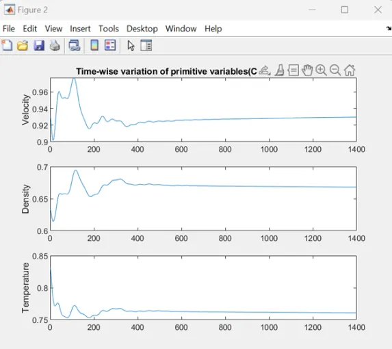
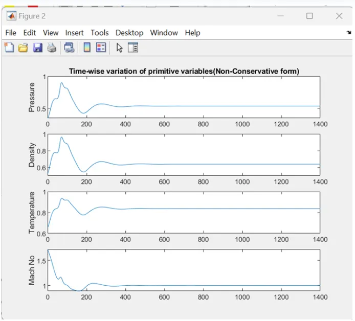
Time-wise Variation at Throat (Figure 2):
- This set of plots shows how velocity, density, and temperature at the throat change over time steps.
- This indicates how the throat conditions stabilize as the simulation progresses.
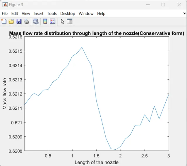
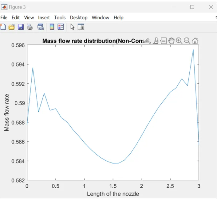
Mass Flow Rate Distribution (Figure 3):
- This plot shows the mass flow rate along the length of the nozzle at the final time step.
- It helps verify the conservation of mass flow rate through the nozzle.
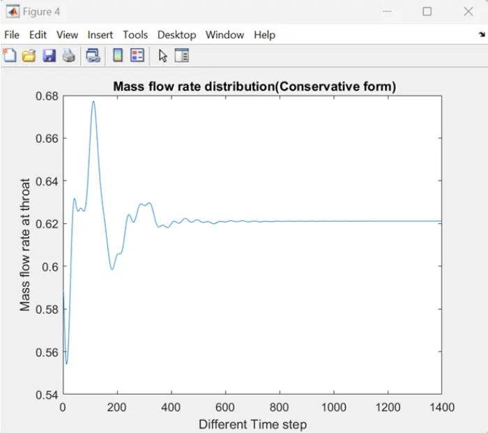
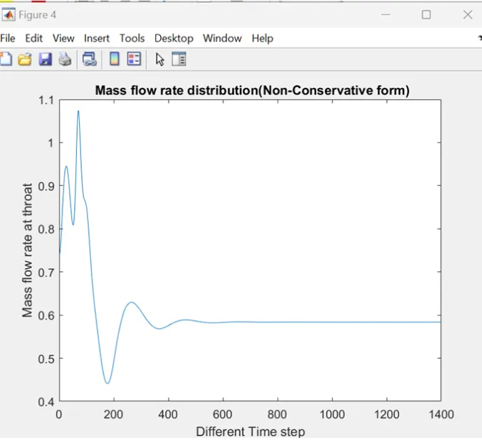
Mass Flow Rate at Throat Over Time (Figure 4):
- This plot shows how the mass flow rate at the throat evolves over time.
- It should stabilize, indicating steady-state conditions.
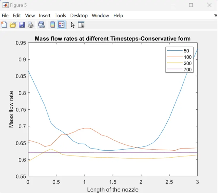
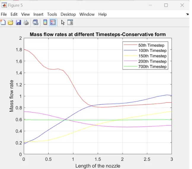
Mass Flow Rates at Different Time Steps (Figure 5):
- This plot shows the mass flow rates at various significant time steps (50, 100, 200, 700, 800, 1000, 1400).
- This demonstrates the progression toward a steady-state mass flow rate distribution through the nozzle.