Week 7 - Simulation of a 1D Supersonic nozzle flow simulation using Macormack Method
WEEK 7- CHALLENGE-DETAILED REPORT
OBJECTIVES:
Simulate the isentropic flow through a quasi 1D subsonic-supersonic nozzle.
Derive both the conservation and non-conservation forms of the governing equations and sovle them using the MacCormack's technique.
Determine the steady-state temperature distribution for the flow-field variables and investigate the difference between the two forms of governing equations by comparing their solutions.
Perform a grid independence test on the solution and expain all your findings.
Understand and derive the conservative and non-conservative form mass conservation, momentum conservation and energy conservation equations.
Specify the initial and boundary conditions for each case.
Create a basic modular code, with function calls for each form of solution and compare the solutions using the primitive variables- mass flow rate, density, pressure, temperature and mach number.
GOVERNING EQUATIONS AND THEORY:
1D Supersonic Nozzle:
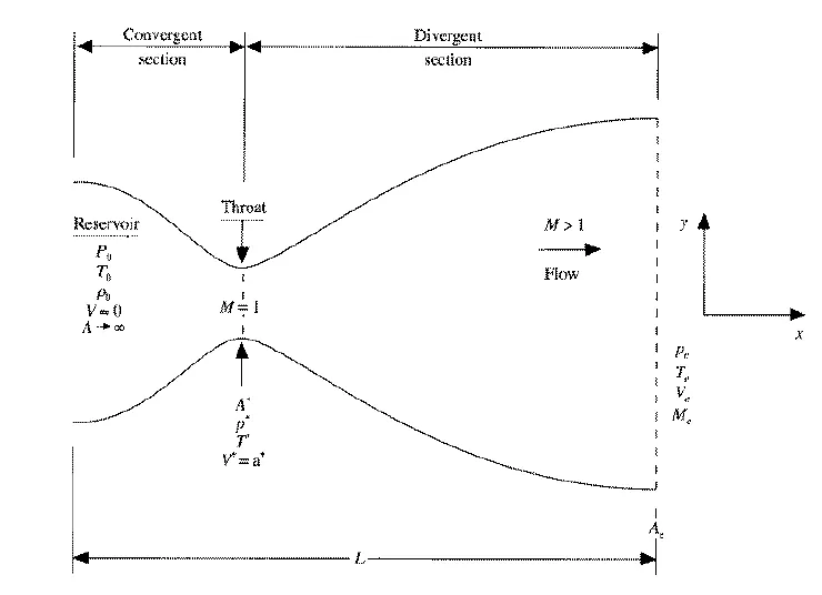
A supersonic nozzle consists of three sections, the convergent part, throat and the divergent part. In the convergent part the fluid is assumed to be entering from a reservoir and consists a Mach nnumber less than 1, therefore the flow is subsonic. At the throat, as the mass flow rate is constant, and area of cross-section decreases, velocity of the fluid increases. This leads to the Mach number reaching sonic flow at Mach number 1. In the divergent section as the area of crossection increase, but the flow variables are changed and maintained such that the flow velocity increase further more to supersonic regime where mach number is greater than 1.
The MacCormack method to be used is an average solution obtained from the weighted solutions of forward and backward differencing of space derivatives in the discretized equations. A time marching solution is used to obtain the solution of the problem, starting from few initial and boundary conditions which will be discussed later. In a time marching solution the current time step calculations are used to guide the way to the next time step solution.
FUNCTION PROGRAMME FOR NON-CONSERVATIVE FORM:
function [x,pr,rho,t,M,m, dummy_m, dummy_M,dummy_pr, dummy_t, dummy_v,dummy_massthroat] = non_conservative(n)
x=linspace(0,3,n); % doing meshing
dx=x(2)-x(1); % calculating distance between two adjacent nodes
gamma=1.4; % giving value for gamma

% calculate initial condition

rho=1-0.3146*x;
t=1-0.2314*x;
v=(0.1+1.09*x).*t.^0.5;
% defing area
a=1+2.2*(x-1.5).^2;
% finding row and coloumn where area becomes one
[r,c]=find(a==1);

% time step
nt=1400;
dt=0.01;


% time loop
for k=1:nt

    % assigning initial values
    rho_old=rho;
    v_old=v;
    t_old=t;
    % predictor method


    for j=2:n-1
        %drho_dt_p=-rho(j)*(v(j+1)-v(j))/dx-(rho(j)*v(j)(loga(j+1)-loga(j))/dx)-v(j)*(rho(j+1)-rho(j))/dx

dvdx=(v(j+1)-v(j))/dx;
drhodx=(rho(j+1)-rho(j))/dx;
dtdx=(t(j+1)-t(j))/dx;
dlogadx=(log(a(j+1))-log(a(j)))/dx;

% writing equations
% continuity equation
drho_dt_p(j)=-rho(j)*dvdx-rho(j)*v(j)*dlogadx-v(j)*drhodx;
% momentum equation
dvdt_p(j)=-v(j)*dvdx-1/gamma*(dtdx+(t(j)/rho(j))*drhodx);
% energy equation
dtdt_p(j)=-v(j)*dtdx-(gamma-1)*t(j)*(dvdx+v(j)*dlogadx);


% solution update
 rho(j)=rho(j)+ drho_dt_p(j)*dt;
  v(j)=v(j)+dvdt_p(j)*dt;
  t(j)=t(j)+dtdt_p(j)*dt;

  end % ending predictor step

   % corrector method


    for j=2:n-1
        %drho_dt_p=-rho(j)*(v(j+1)-v(j))/dx-(rho(j)*v(j)(loga(j+1)-loga(j))/dx)-v(j)*(rho(j+1)-rho(j))/dx

dvdx=(v(j)-v(j-1))/dx;
drhodx=(rho(j)-rho(j-1))/dx;
dtdx=(t(j)-t(j-1))/dx;
dlogadx=(log(a(j))-log(a(j-1)))/dx;

% writing equations
% continuity equation
drho_dt_c(j)=-rho(j)*dvdx-rho(j)*v(j)*dlogadx-v(j)*drhodx;
% momentum equation
dvdt_c(j)=-v(j)*dvdx-1/gamma*(dtdx+(t(j)/rho(j))*drhodx);
% energy equation
dtdt_c(j)=-v(j)*dtdx-(gamma-1)*t(j)*(dvdx+v(j)*dlogadx);


  end % ending corrector step

  % compute the average time derivative
  drhodt=0.5*(drho_dt_p+drho_dt_c);
  dvdt=0.50*(dvdt_p+dvdt_c);
  dtdt=0.5*(dtdt_p+dtdt_c);
  for i=2:n-1
  % final solution update
  rho(i)=rho_old(i)+drhodt(i)*dt;
   v(i)=v_old(i)+dvdt(i)*dt;
    t(i)=t_old(i)+dtdt(i)*dt;
  end
    % define pressure,Mach number and mass flow rate
    pr=rho.*t;
    M=v./sqrt(t);
    m=rho.*a.*v;
    % calculating primitive variables for all columns and for all time
    % steps
    dummy_m(k,:)=m;
    dummy_M(k)=M(c);
    dummy_pr(k)=pr(c);
    dummy_t(k)=t(c);
    dummy_v(k)=v(c);
    dummy_massthroat(k)=m(c);

    % apply boundary condition
    % inlet
   v(1)=2*v(2)-v(3);
   %outlet
   v(n)=2*v(n-1)-v(n-2);
   rho(n)=2*rho(n-1)-rho(n-2);
   t(n)=2*t(n-1)-t(n-2);

   figure(1)

   if k==50
       plot(x,m)
   end
   hold on
    if k==100
       plot(x,m)
    end
    if k==150
       plot(x,m)
    end
    if k==200
       plot(x,m)
    end
    if k==700
       plot(x,m)
   end
end


title('mass flow rate at diiferent time step non conservative');
legend('50','100','150','200','700');
xlabel('x(length of nozzle)')
ylabel('mass flow rate')


end
FUNCTION PROGRAMME FOR CONSERVATIVE FORM:
function [x,pr,rho,t,M,m,m_t,rho_t,v_t,t_t,pr_t,M_t] = conservative(n)

x=linspace(0,3,n);
dx=x(2)-x(1);
gamma=1.4;
a=1+2.2*(x-1.5).^2;
throat = find(a==1);


% calculate initial condition
for i=1:length(x)
    if x(i)>=0 && x(i)<=0.5
        rho(i)=1;
        t(i)=1;
    end
    if x(i)>=0.5 && x(i)<=1.5
        rho(i)=1-0.366*(x(i)-0.5);
        t(i)=1-0.167*(x(i)-0.5);
    end
    if x(i)>=1.5 && x(i)<=3.5
        rho(i)=0.634-0.3879*(x(i)-1.5);
        t(i)=0.833-0.3507*(x(i)-1.5);
    end

end


v=0.59./(rho.*a);

pr=rho.*t;

rho_initial=rho;
t_initial=t;
v_initial=v;
cfl=0.5; % Courant number

% time step
nt=1400;


U1=rho.*a;
U2=rho.*a.*v;
U3=rho.*a.*( (t./(gamma-1))+(gamma/2)*v.^2);


% time loop
for k=1:1400

    U1_old=U1;
    U2_old=U2;
    U3_old=U3;

    dt=min(abs((cfl*dx)./(sqrt(t)+v)));% defining dt

    % predictor method

    % defining F1,F2 and F3
    F1 = U2;
    F2 = (U2.^2)./U1 + ((gamma-1)/gamma)*( U3 - (gamma/2)*(U2.^2)./U1 );
    F3 = gamma*U2.*U3./U1 - (gamma*(gamma-1)/2)*(U2.^3)/(U1.^2);

    for j=2:(n-1)
        % defining J2
        J2(j)=(1/gamma)*rho(j).*t(j).*((a(j+1)-a(j))/dx);
        % defining equations
        dU1_dt_p(j) = -(F1(j+1)-F1(j))/dx;

        dU2_dt_p(j) = -((F2(j+1)-F2(j))/dx)+J2(j);

        dU3_dt_p(j) = -(F3(j+1)-F3(j))/dx;

% solution update (updating U1,U2 and U3)
U1(j)=U1(j)+dU1_dt_p(j)*dt;

  U2(j)=U2(j)+dU2_dt_p(j)*dt;

  U3(j)=U3(j)+dU3_dt_p(j)*dt;


   end % ending predictor step


   rho=U1./a;
    v=U2./U1;
    t=(gamma-1)*(U3./U1- (gamma/2)*v.^2);
    %pr=rho.*t;
  % updating F1,F2 anf  F3
    F1=U2;
    F2=(U2.^2./U1)+((gamma-1)/gamma)*(U3-(gamma*U2.^2)./(2*U1));
    F3=(gamma*U2.*U3./U1)-(gamma*(gamma-1)/2)*(U2.^3./U1.^2);


   % corrector method


    for j=2:(n-1)

    % updating J2 by using reverse differencing
        J2(j)=(1/gamma)*rho(j).*t(j).*((a(j)-a(j-1))/dx);

        % defining equations
        dU1_dt_c(j)= -(F1(j)-F1(j-1))/dx;

        dU2_dt_c(j)= -((F2(j)-F2(j-1))/dx)+J2(j);

        dU3_dt_c(j)= -(F3(j)-F3(j-1))/dx;

    end % ending corrector step


  % compute the average time derivative
   dU1_dt=0.5*(dU1_dt_p+dU1_dt_c);
  dU2_dt=0.5*(dU2_dt_p+dU2_dt_c);
    dU3_dt=0.5*( dU3_dt_p+ dU3_dt_c);

  for i=2:(n-1)
  % final solution update
  U1(i)=U1_old(i)+dU1_dt(i)*dt;
   U2(i)=U2_old(i)+ dU2_dt(i)*dt;
  U3(i)=U3_old(i)+ dU3_dt(i)*dt;
  end
  % apply inlet boundary conditions
        U1(1)=rho(1).*a(1);
        U2(1)=2*U2(2)-U2(3);
        U3(1)=U1(1).*((t(1)/(gamma-1))+((gamma/2)*v(1).^2));

  % apply outlet boundary conditions

  U1(n)=2*U1(n-1)-U1(n-2);
  U2(n)=2*U2(n-1)-U2(n-2);
  U3(n)=2*U3(n-1)-U3(n-2);

  % updating primitive variables
    rho=U1./a;
    v=U2./U1;
    t=(gamma-1)*(U3./U1-(gamma/2)*v.^2);

    % define pressure,Mach number and mass flow rate
        M = v./sqrt(t);
        m =rho.*a.*v;
        pr=rho.*t;

    m_t(k) =m(throat);
    rho_t(k) = rho(throat);
    v_t(k) = v(throat);
    t_t(k) = t(throat);
    pr_t(k) = pr(throat);
    M_t(k) = M(throat);
%
%         dummy_M(k)=M(c);
%     dummy_pr(k)=pr(c);
%     dummy_t(k)=t(c);
%     dummy_v(k)=v(c);
%     dummy_massthroat(k)=m(c);


figure(5)

   if k==50
       plot(x,m)
   end
   hold on
    if k==100
       plot(x,m)
    end
    if k==150
       plot(x,m)
    end
    if k==200
       plot(x,m)
    end
    if k==700
       plot(x,m)
    end
end
title('mass flow rate at diiferent time step conservative');
legend('50','100','150','200','700');
xlabel('x(length of nozzle)')
ylabel('mass flow rate')
end
MAIN PROGRAMME:
clear all; % clearing workspace
close all % closing all figures and plots
clc % clearing screen
n=31; % defining number of nodes

% function call for non-conservative case
[x_nc,pr_nc,rho_nc,t_nc,M_nc,m_nc, dummy_m_nc, dummy_M_nc,dummy_pr_nc, dummy_t_nc, dummy_v_nc,dummy_massthroat_nc] = non_conservative(n)

[x_c,pr_c,rho_c,t_c,M_c,m_c,m_t_c,rho_t_c,v_t_c,t_t_c,pr_t_c,M_t_c] = conservative(n);

figure(2)

subplot(4,1,1);
plot(x_nc,pr_nc);
hold on;
plot(x_c,pr_c);
legend('non conservative','consrvative');
xlabel('x(length of nozzle)'); % giving naming to x axis
ylabel('pressure');  % giving naming to y axis
title('variation of primitive variables'); % giving title

subplot(4,1,2);
plot(x_nc,rho_nc)
hold on;
plot(x_c,rho_c);
xlabel('x(length of nozzle)');% giving naming to x axis
ylabel('density'); % giving naming to y axis
legend('non conservative','consrvative');

subplot(4,1,3);
plot(x_nc,t_nc);
hold on;
plot(x_c,t_c);
xlabel('x(length of nozzle)');% giving naming to x axis
ylabel('temperature');% giving naming to y axis

subplot(4,1,4);
plot(x_nc,M_nc);
hold on;
plot(x_c,M_c);
xlabel('x(length of nozzle)');% giving naming to x axis
ylabel('Mach Number');% giving naming to y axis
legend('non conservative','consrvative');

figure(3)

plot(x_nc,m_nc);
hold on;
plot(x_c,m_c);
title('variation of mass flow rate with length of nozzle');% giving title
legend('non conservative','consrvative');

figure(4)

subplot(5,1,1);

plot(dummy_M_nc);
hold on;
plot(M_t_c)
title('primitive varialbe at throat for all time step');% giving title
xlabel('time step'); % giving naming to x axis
ylabel('Mach Number'); % giving naming to y axis
legend('non conservative','conservative');

subplot(5,1,2)

plot(dummy_pr_nc);
hold on;
plot( pr_t_c)
xlabel('time step'); % giving naming to x axis
ylabel('pressure');  % giving naming to y axis
legend('non conservative','conservative');


subplot(5,1,3)

plot(dummy_t_nc);
hold on;
plot( t_t_c);
xlabel('time step');% giving naming to x axis
ylabel('temperature'); % giving naming to y axis
legend('non conservative','conservative');

subplot(5,1,4)

plot(dummy_v_nc);
hold on;
 plot( v_t_c);
xlabel('time step');% giving naming to x axis
ylabel('velocity'); % giving naming to y axis
legend('non conservative','conservative');

subplot(5,1,5)

plot(dummy_massthroat_nc);
hold on;
plot(m_t_c);
xlabel('time step');% giving naming to x axis
ylabel('mass flow rate'); % giving naming to y axis
legend('non conservative','conservative');
MAIN PLOTS ARE GIVEN BELOW:
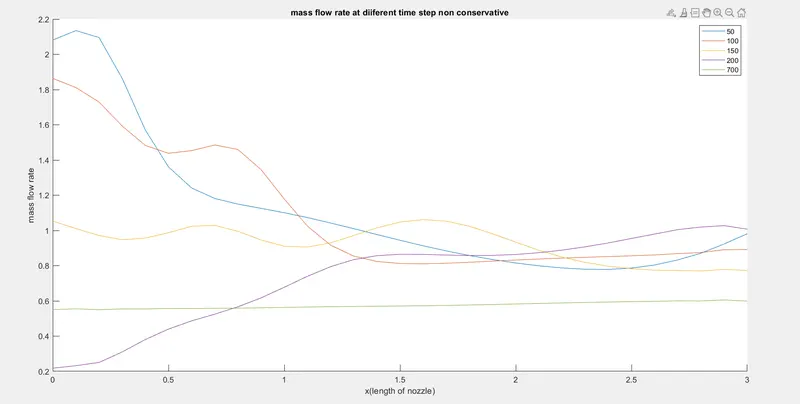
Plot for mass flow rate at different time step for non-conservative form
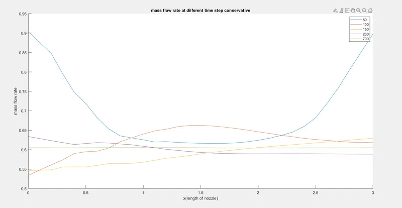
Plot for mass flow rate at different time step for conservative form
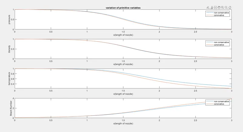
Plot for the variation of primitive variables for both conservative and non-conservative forms.
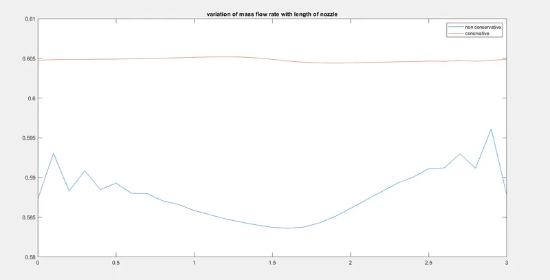
PLOT FOR THE VARIATION OF MASS FLOW RATE WITH LENGTH OF NOZZLE FOR CONSERVATIVE AND NON-CONSERVATIVE FORM
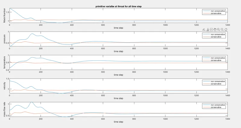
PLOT FOR THE VARIATION OF PRIMITIVE VARIABLES AT THE THROAT FOR CONSERVATIVE AND NON-CONSERVATIVE FORM
CONCLUSIONS:
* In conservative form control volume will not move and conservative volume also known as Eulers approach.
*In non- conservative form control volume will move and non-conservative volume also known as Lagragian approach.
*In non-conservative form as well as in conservative form mass flow rate will become constant at 700th time step.
*There is no much differences in the variation of primitive variables in both non-conservative form and in conservative form
*When we are comparing onservative form and non-conservative form, fluctuation of mass flow rate is more in non-conservative form and it is clear from 3rd plot
*There is no much differences in the variation of primitive variables at the throat also in both non-conservative form and in conservative form