Week 7 - Simulation of a 1D Supersonic nozzle flow simulation using Macormack Method
The conservation and non-conservation equations of motion using the Maccormack technique are derived on paper and uploaded as PDF.
After the derivations, the codes are developed with the help of a project help video. For the non-conservation, it is pretty much straightforward to develop. But for conservation, the project help video is more helpful. Initially, I did the code for non-conservation and conservation for one n_value which is 31(no.of grid points).
Here is the code developed for both Non-conservation and conservation equations as functions
clear
close all
clc

% Based on CFD book input parameters
l =3;
n_values=[31];
nt=1:1400;
cfl=0.5;

for i = 1:length(n_values)
    x=linspace(0,l,n_values(i));
    [m_fr_nc,m_fr_at_throat_nc] =non_conservative_form(l,n_values(i),nt,cfl);
   [m_fr_c,m_fr_at_throat_c] =conservative_form(l,n_values(i),nt,cfl);

%Plot the comparision of Non-conservation and Conservation mass flow rate
figure(7)
plot(nt, m_fr_at_throat_c,'r',nt, m_fr_at_throat_nc, 'b', 'linewidth', 2)
xlabel('Time steps (nt)')
ylabel('Mass flow rate')
legend('Conservative form', 'Non-Conservative form')
title('Mass flow rate using "Non-Conservative form vs Conservative form" at throat point i=16')

figure(8)
plot(x,m_fr_c,'b',x,m_fr_nc,'r','linewidth',2)
xlabel('Length of nozzle')
ylabel('Mass flow rate')
legend('Conservative form','Non-Conservative form')
title('Mass flow rate using "Non-Conservative form vs Conservative form" in the nozzle')

end


function [m_fr_nc,m_fr_at_throat_nc]=non_conservative_form(l, n_values, nt, cfl)
 x=linspace(0, l, n_values);
 dx = x(2) - x(1);

%Initial conditions rho, a, v, T, mfr, M, p
rho =1-0.3146*x;                 %density
t =1-0.2314*x;                      % temperature
v=(0.1+0.9*x).*t.^0.5;         % veloocity

%Area based on Eq7.73 from Anderson book
a =1+2.2*(x-1.5).^2;

%Mach number
M = v./(t.^0.5);
p=rho.*t;
m_fr = rho.* a.*v;

gamma =1.4;

dt = zeros(1, n_values);
for k =1:31
      u = ((t(k)))^(0.5);
    dt(k) = cfl * dx / (u + v(k));
end
dt = min(dt);

for i = 1:length(nt)
    %storing initial values
    rho_old=rho;
    t_old = t;
    v_old = v;
for j = 2:n_values-1

         %Predictor step
         drho_dx =(rho(j+1)-rho(j))/dx;
         dv_dx = (v(j+1) - v(j)) / dx;
         dt_dx = (t(j+1) - t(j)) / dx;
         da_dx = (log(a(j+1)) - log(a(j))) / dx;

         drho_dt_p(j) = -rho(j) * dv_dx - rho(j) * v(j) * da_dx - v(j) * drho_dx;   % continuity
        dv_dt_p(j) = -v(j) * dv_dx - (1/gamma) * (dt_dx + (t(j) / rho(j)) * drho_dx);     % momentum
        dt_dt_p(j) = -v(j) * dt_dx - (gamma - 1) * t(j) * (dv_dx + v(j) * da_dx);    % energy

        %Updating the Primitive variables
        v(j) = v_old(j) + dv_dt_p(j) *dt;
        rho(j) = rho_old(j) + drho_dt_p(j) *dt;
        t(j) = t_old(j) + dt_dt_p(j) *dt;

        % corrector step
        drho_dx = (rho(j) - rho(j-1)) / dx;
        dv_dx = (v(j) - v(j-1)) / dx;
        dt_dx = (t(j) - t(j-1)) / dx;
        da_dx = (log(a(j)) - log(a(j-1))) / dx;

        drho_dt_c(j) = -rho(j) * dv_dx - rho(j) * v(j) * da_dx - v(j) * drho_dx;   % continuity
        dv_dt_c(j) = -v(j) * dv_dx - (1/gamma) * (dt_dx + (t(j) / rho(j)) * drho_dx);     % momentum
        dt_dt_c(j) = -v(j) * dt_dx - (gamma - 1) * t(j) * (dv_dx + v(j) * da_dx);    % energy
end
   % average time derivatives
    drho_dt_avg =  (drho_dt_p + drho_dt_c)/2;
    dv_dt_avg =  (dv_dt_p + dv_dt_c)/2;
    dt_dt_avg =  (dt_dt_p + dt_dt_c)/2;

% final corrected values
    for k = 2:n_values-1
        rho(k) = rho_old(k) + drho_dt_avg(k) * dt;
        v(k) = v_old(k) + dv_dt_avg(k) * dt;
        t(k) = t_old(k) + dt_dt_avg(k) * dt;
    end
    % entry boundary conditions
    v(1) = 2 * v(2) - v(3);

    % exit boundary conditions
    v(n_values) = 2 * v(n_values-1) - v(n_values-2);
    rho(n_values) = 2 * rho(n_values-1) - rho(n_values-2);
    t(n_values) = 2 * t(n_values-1) - t(n_values-2);

 % Final update of primitives
    p = rho .* t;
    M = v ./ t.^0.5;
    mfr = rho .* a .* v;

 % to find values at throat point
    rho_throat(i) = rho(16);
    v_throat(i) = v(16);
     t_throat(i) = t(16);
    M_throat(i) = M(16);
    p_throat(i) = p(16);
    mfr_throat(i) = mfr(16);

    % plotting mass flow rate at specific iterations
    if n_values == 31
        for ii = [1:50:201 700]
            if ii == i
                figure(1)
                plot(x, mfr, 'linewidth', 2.0)
                hold on
                title('Non-Conservative form - Variation of Mass flow rate distribution inside the nozzle at different time steps ')
                xlabel('Length of nozzle')
                ylabel('Mass flow rate')
            elseif i == 1000
                plot(x, mfr, '*b')
                legend('At 1', 'At 51', 'At 101', 'At 151', 'At 201', 'At 700', 'At 1000')
            end
        end
    end
end

if n_values == 31
    figure(2)
    plot(x, v, 'r', x, p, 'b', x, t, 'm', x, rho, 'g', x, M, 'k', x, mfr, 'c')
    xlim([0 3.0])
    ylim([0 3.5])
   title(['Time step = ' num2str(i)])
    xlabel('Length of nozzle')
    ylabel('Non dimensional parameters')
    legend('Velocity', 'Pressure', 'Temperature', 'Density', 'Mach number', 'Mass flow rate', 'location', 'northwest')
    title('Non-Conservative form - Steady-state distribution of primitive variables inside the nozzle')

    figure(3)
    plot(nt, rho_throat)
    hold on
    plot(nt, v_throat, 'linewidth', 2)
    plot(nt, p_throat, 'linewidth', 2)
    plot(nt, t_throat, 'linewidth', 2)
    plot(nt, M_throat, 'linewidth', 2)
    plot(nt, mfr_throat, 'linewidth', 2)
    xlabel('Time steps (nt)')
    ylabel('Non dimensional parameters')
    legend('Density', 'Velocity', 'Pressure', 'Temperature', 'Mach number', 'Mass flow rate')
    title('Non-Conservative form- variation of the primitive variables at throat point i=16')
end
m_fr_nc = mfr;
m_fr_at_throat_nc = mfr_throat;
end

function [m_fr_c,m_fr_at_throat_c] =conservative_form(l, n_values, nt, cfl)
 x=linspace(0, l, n_values);
 dx = x(2) - x(1);


 %Initial conditions
  for kk=1:length(x)
      if (x(kk)<=0.5)
          rho(kk) =1;
          t(kk) =1;

      elseif (x(kk)>0.5) & (x(kk)<=1.5)
          rho(kk) =1.0-0.366*(x(kk)-0.5);
          t(kk) = 1.0-0.167*(x(kk)-0.5);

      elseif (x(kk)>1.5) & (x(kk)<=3.5)
          rho(kk) =0.634-0.3879*(x(kk)-1.5);
          t(kk) = 0.833-0.3507*(x(kk)-1.5);
      end
  end

  %Nozzle area and gamma
  a = 1 +2.2*(x-1.5).^2;
  gama =1.4;

  %Solution variable initialization
  u1 = rho.*a;
  u2 = 0.59*ones(1,n_values);
  v =u2./u1;
  u3 = u1.*((t./(gama-1))+(gama/2).*v.^2)

 M= v./(t.^0.5);           %mach number
 mfr = rho.*a.*v;        %mass flow rate
  p=rho.*t;                   %pressure

  %Time step evaluation using CFL
  for k =1:31
  u =(t(k))^(0.5);
 dt(k) = cfl*dx/(u+v(k));
  end
  dt = min(dt);

  for i = 1: length(nt)
    % Storing initial values
     u1_old =u1;
     u2_old =u2;
     u3_old =u3;

     for j = 2: n_values-1

        % Define flux vectors
          f1 = u2;
          f2 = ((u2.^2)./u1)+((gama-1)/gama)*(u3-((gama/2)*(u2.^2)./u1));
         f3 = ((gama.*u2.*u3)./u1) - ((gama*(gama-1)/2)*(u2.^3)./(u1.^2));

       % Source term
       j1 = (1/gama)*rho(j)*t(j)*((a(j+1)-a(j))/dx);

     %predictor step
        du1_dt_p(j)= -(f1(j+1)-f1(j))/dx;            %continuity
        du2_dt_p(j)= -(f2(j+1)-f2(j))/dx + j1;     %momentum
        du3_dt_p(j)= -(f3(j+1)-f3(j))/dx;            %energy
     %updating solution vectors
        u1(j) = u1_old(j) + du1_dt_p(j)*dt;
        u2(j) = u2_old(j) + du2_dt_p(j)*dt;
        u3(j) = u3_old(j) + du3_dt_p(j)*dt;
   %updating primitives
        rho=u1./a;
        t=(gama-1).*(u3./u1-(gama/2).*(u2./u1).^2);
    % updating flux terms
        f1=u2;
        f2=u2.^2./u1+((gama-1)/gama).*(u3-(gama/2)*u2.^2./u1);
        f3=gama.*u2.*u3./u1-0.5*gama*(gama-1).*u2.^3./u1.^2;


   %source term for corrector step
        j2 = (1/gama)*(rho(j)*t(j)*(a(j)-a(j-1))/dx);

   %corrector step
        du1_dt_c(j) = -(f1(j)-f1(j-1))/dx;            %continuity
        du2_dt_c(j) = -(f2(j)-f2(j-1))/dx + j2;       %momentum
        du3_dt_c(j) = -(f3(j)-f3(j-1))/dx;            %energy
     end

       %Final time derivatives
        du1_dt_avg = (du1_dt_p + du1_dt_c)/2;
        du2_dt_avg = (du2_dt_p + du2_dt_c)/2;
        du3_dt_avg = (du3_dt_p + du3_dt_c)/2;

% final corrected values
    for k = 2:n_values-1
        u1(k) = u1_old(k) + du1_dt_avg(k) * dt;
        u2(k) = u2_old(k) + du2_dt_avg(k) * dt;
        u3(k) = u3_old(k) + du3_dt_avg(k) * dt;
    end

    % Boundary conditions
        u1(1) = a(1);
        u2(1) = 2*u2(2)-u2(3);
        u3(1) = u1(1)*(t(1)/(gama-1) + (gama*(u2(1)/u1(1))^2)/2);

        u1(n_values) = 2*u1(n_values-1)-u1(n_values-2);
        u2(n_values) = 2*u2(n_values-1)-u2(n_values-2);
        u3(n_values) = 2*u3(n_values-1)-u3(n_values-2);

%Final update for primitive variables
        rho = u1./a;
        v = u2./u1;
        t=(gama-1).*(u3./u1-(gama/2).*(u2./u1).^2);
        p = rho.*t;
        M= v./t.^0.5;
        error(k) =  abs(v(k)-v(k-1));
        mfr= u2;

        % For the case of throat

    rho_throat(i) = rho(16);
    v_throat(i) = v(16);
    t_throat(i) = t(16);
    M_throat(i) = M(16);
    p_throat(i) = p(16);
    mfr_throat(i) = mfr(16);

% plotting mass flow rate at specific iterations
    if n_values == 31
        for ii = [1:50:201 700]
            if ii == i
                figure(4)
                plot(x, mfr, 'linewidth', 2.0)
                hold on
                title('Conservative form - Variation of Mass flow rate distribution inside the nozzle at different time steps ')
                xlabel('Length of nozzle')
                ylabel('Mass flow rate')
            elseif i == 1000
                plot(x, mfr, '*b')
                legend('At 1', 'At 51', 'At 101', 'At 151', 'At 201', 'At 700', 'At 1000')
            end
        end
    end
end

if n_values == 31
    figure(5)
    plot(x, v, 'r', x, p, 'b', x, t, 'm', x, rho, 'g', x, M, 'k', x, mfr, 'c')
    xlim([0 3.0])
    ylim([0 3.5])
   title(['Time step = ' num2str(i)])
    xlabel('Length of nozzle')
    ylabel('Non dimensional parameters')
    legend('Velocity', 'Pressure', 'Temperature', 'Density', 'Mach number', 'Mass flow rate', 'location', 'northwest')
    title('Conservative form - Steady-state distribution of primitive variables inside the nozzle')

    figure(6)
    plot(nt, rho_throat)
    hold on
    plot(nt, v_throat, 'linewidth', 2.0)
    plot(nt, p_throat, 'linewidth', 2.0)
    plot(nt, t_throat, 'linewidth', 2.0)
    plot(nt, M_throat, 'linewidth', 2.0)
    plot(nt, mfr_throat, 'linewidth', 2.0)
    xlabel('Time steps (nt)')
    ylabel('Non dimensional parameters')
    legend('Density', 'Velocity', 'Pressure', 'Temperature', 'Mach number', 'Mass flow rate')
    title('Conservative form - variation of the primitive variables at throat point i=16')
end
m_fr_c = mfr;
m_fr_at_throat_c = mfr_throat;
end
which will give an output for the
Figure 1:Non-Conservative form - Variation of Mass flow rate distribution inside the nozzle at different time steps
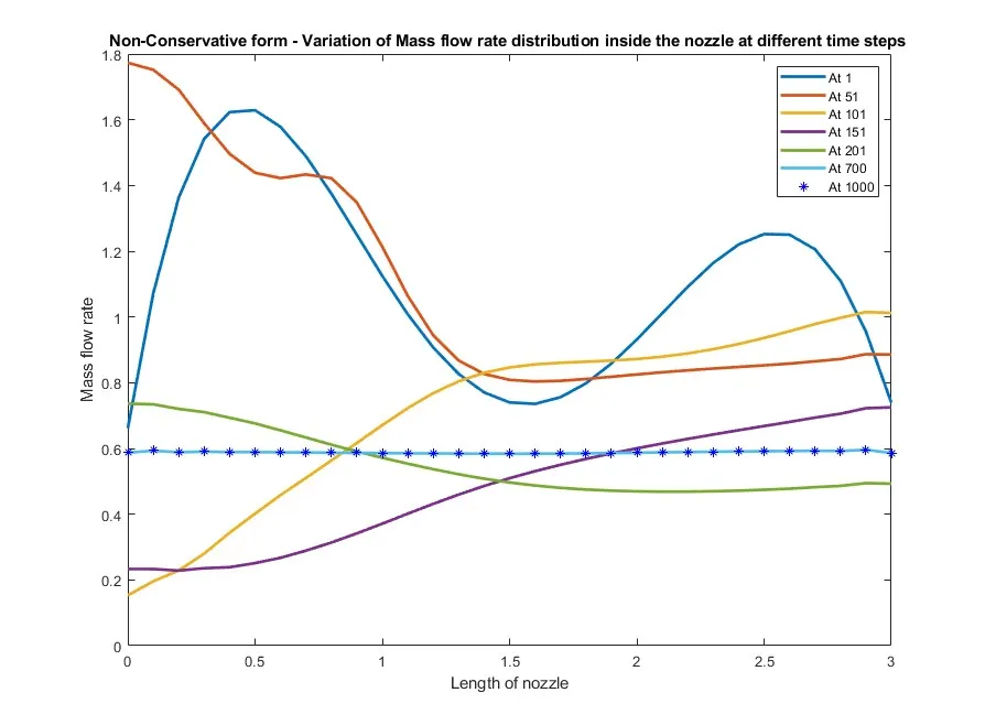
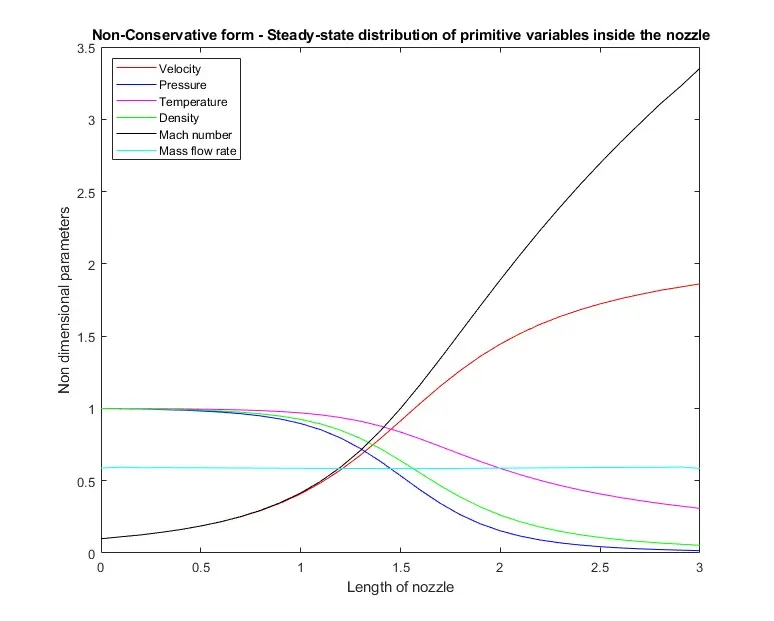
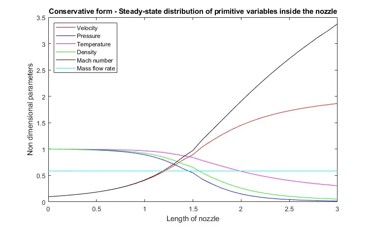
Fig 2 Non-Conservative form - Steady-state distribution of primitive variables inside the nozzle
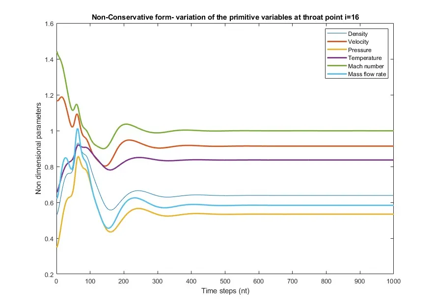
Fig 3 Non-Conservative form- variation of the primitive variables at throat point i=16
For the case of conservation, the graphs are as follows.
Fig.4 Conservative form - Variation of Mass flow rate distribution inside the nozzle at different time steps
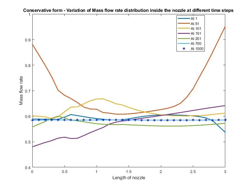
Fig 5 Conservative form - Steady-state distribution of primitive variables inside the nozzle
Fig 6 Conservative form - variation of the primitive variables at throat point i=16
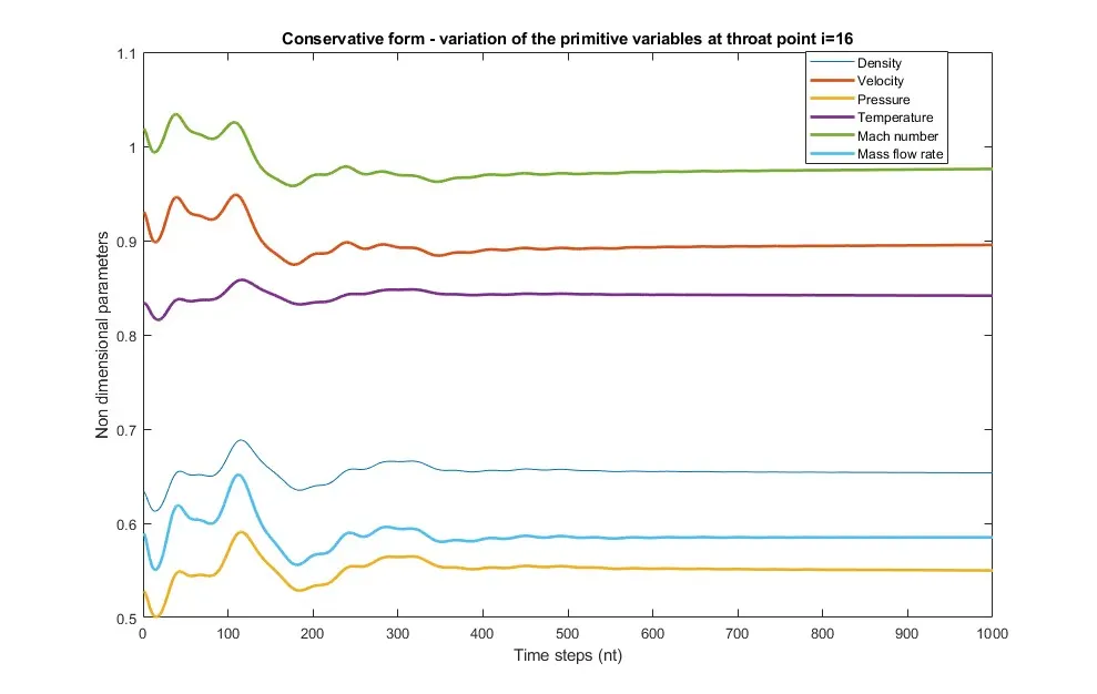
If we look at the mass flow rate between non-conservation and conservation forms we can observe that the solution becomes more stable within lesser steps in the conservation form compared to the Non-Conservation form.
Also in the case throat section after the No. of steps reaching between 400-500, the properties attain a steady state. This means that the solution converges within these time steps.
For the comparison of Non-conservation and conservation forms mass flow rate at the throat section and in the nozzle created graphs in the main code.
So these are the outputs for the comparison of the mass flow rate
Fig 7 Mass flow rate "Non-Conservative form vs Conservative form" at throat
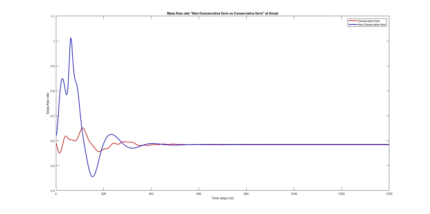
If we compare the mass flow rate between the two forms initially the mass flow rate is different but after a certain no. of steps (~500)the mass flow rate reaches a steady state in each form. The Conservative form reaches a steady state quicker than the non-conservative form.
Fig 8 Mass flow rate "Non-Conservative form vs Conservative form" in the Nozzle
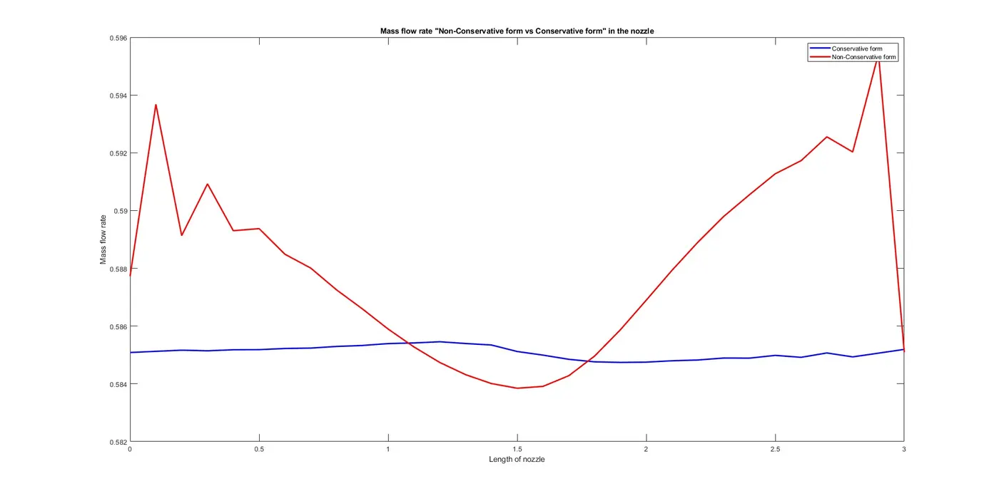
The mass flow rate in the nozzle also between both forms revolves around 0.588±5 but pretty much stays constant in the conservation form except at the initial and final sections of the non-conservation form. From Fig 7 and 8, we can conclude that both method works fine. each method has its own advantages and disadvantages.
conservation method with fewer time steps and longer time and non-conservation with vice versa.
After this, For the case of the grid independence study, I am using different n_values for the comparison.For plots 9 and 10 i used the following code to compare the grid independence study and along the throat and in the nozzle.
clear
close all
clc

% Based on CFD book input parameters
l =3;
n_values=[31 62 93];
nt=1:1400;
cfl=0.5;

for i = 1:length(n_values)
    x=linspace(0,l,n_values(i));
    [m_fr_nc,m_fr_at_throat_nc] =non_conservative_form(l,n_values(i),nt,cfl);
   [m_fr_c,m_fr_at_throat_c] =conservative_form(l,n_values(i),nt,cfl);

% %Plot the comparision of Non-conservation and Conservation mass flow rate
% figure(7)
% plot(nt, m_fr_at_throat_c,'r',nt, m_fr_at_throat_nc, 'b', 'linewidth', 2)
% xlabel('Time steps (nt)')
% ylabel('Mass flow rate')
% legend('Conservative form', 'Non-Conservative form')
% title('Mass flow rate using "Non-Conservative form vs Conservative form" at throat point i=16')
%
% figure(8)
% plot(x,m_fr_c,'b',x,m_fr_nc,'r','linewidth',2)
% xlabel('Length of nozzle')
% ylabel('Mass flow rate')
% legend('Conservative form','Non-Conservative form')
% title('Mass flow rate using "Non-Conservative form vs Conservative form" in the nozzle')

figure(9)
subplot (2,1,1)
plot(nt,m_fr_at_throat_c,'linewidth',2)
hold on
xlabel('Time steps (nt)')
ylabel('Mass flow rate')
legend('@31 nodes','@61 nodes','@92 nodes')
title('Conservative form: Grid independency test at throat')
subplot (2,1,2)
plot(nt,m_fr_at_throat_nc,'linewidth',2)
hold on
xlabel('Time steps (nt)')
ylabel('Mass flow rate')
legend('@31 nodes','@61 nodes','@92 nodes')
title('Non-Conservative form: Grid independency test at throat ')

figure(10)
subplot (2,1,1)
plot(x,m_fr_c,'linewidth',2)
hold on
xlabel('Length of nozzle')
ylabel('Mass flow rate')
legend('@31 nodes','@61 nodes','@92 nodes')
title('Conservative form: Grid independency test along the nozzle')
subplot (2,1,2)
plot(x,m_fr_nc,'linewidth',2)
hold on
xlabel('Length of nozzle')
ylabel('Mass flow rate')
legend('@31 nodes','@61 nodes','@92 nodes')
title('Non-Conservative form: Grid independency test along the nozzle')
end

function [m_fr_nc,m_fr_at_throat_nc]=non_conservative_form(l, n_values, nt, cfl)
 x=linspace(0, l, n_values);
 dx = x(2) - x(1);

%Initial conditions rho, a, v, T, mfr, M, p
rho =1-0.3146*x;                 %density
t =1-0.2314*x;                      % temperature
v=(0.1+1.09*x).*t.^0.5;         % veloocity

%Area based on Eq7.73 from Anderson book
a =1+2.2*(x-1.5).^2;

%Mach number
M = v./(t.^0.5);
p=rho.*t;
m_fr = rho.* a.*v;

gamma =1.4;

dt = zeros(1, n_values);
for k =1:31
      u = ((t(k)))^(0.5);
    dt(k) = cfl * dx / (u + v(k));
end
dt = min(dt);

for i = 1:length(nt)
    %storing initial values
    rho_old=rho;
    t_old = t;
    v_old = v;
for j = 2:n_values-1

         %Predictor step
         drho_dx =(rho(j+1)-rho(j))/dx;
         dv_dx = (v(j+1) - v(j)) / dx;
         dt_dx = (t(j+1) - t(j)) / dx;
         da_dx = (log(a(j+1)) - log(a(j))) / dx;

         drho_dt_p(j) = -rho(j) * dv_dx - rho(j) * v(j) * da_dx - v(j) * drho_dx;   % continuity
        dv_dt_p(j) = -v(j) * dv_dx - (1/gamma) * (dt_dx + (t(j) / rho(j)) * drho_dx);     % momentum
        dt_dt_p(j) = -v(j) * dt_dx - (gamma - 1) * t(j) * (dv_dx + v(j) * da_dx);    % energy

        %Updating the Primitive variables
        v(j) = v_old(j) + dv_dt_p(j) *dt;
        rho(j) = rho_old(j) + drho_dt_p(j) *dt;
        t(j) = t_old(j) + dt_dt_p(j) *dt;

        % corrector step
        drho_dx = (rho(j) - rho(j-1)) / dx;
        dv_dx = (v(j) - v(j-1)) / dx;
        dt_dx = (t(j) - t(j-1)) / dx;
        da_dx = (log(a(j)) - log(a(j-1))) / dx;

        drho_dt_c(j) = -rho(j) * dv_dx - rho(j) * v(j) * da_dx - v(j) * drho_dx;   % continuity
        dv_dt_c(j) = -v(j) * dv_dx - (1/gamma) * (dt_dx + (t(j) / rho(j)) * drho_dx);     % momentum
        dt_dt_c(j) = -v(j) * dt_dx - (gamma - 1) * t(j) * (dv_dx + v(j) * da_dx);    % energy
end
   % average time derivatives
    drho_dt_avg =  (drho_dt_p + drho_dt_c)/2;
    dv_dt_avg =  (dv_dt_p + dv_dt_c)/2;
    dt_dt_avg =  (dt_dt_p + dt_dt_c)/2;

% final corrected values
    for k = 2:n_values-1
        rho(k) = rho_old(k) + drho_dt_avg(k) * dt;
        v(k) = v_old(k) + dv_dt_avg(k) * dt;
        t(k) = t_old(k) + dt_dt_avg(k) * dt;
    end
    % entry boundary conditions
    v(1) = 2 * v(2) - v(3);

    % exit boundary conditions
    v(n_values) = 2 * v(n_values-1) - v(n_values-2);
    rho(n_values) = 2 * rho(n_values-1) - rho(n_values-2);
    t(n_values) = 2 * t(n_values-1) - t(n_values-2);

 % Final update of primitives
    p = rho .* t;
    M = v ./ t.^0.5;
    mfr = rho .* a .* v;

 % to find values at throat point
    rho_throat(i) = rho(16);
    v_throat(i) = v(16);
     t_throat(i) = t(16);
    M_throat(i) = M(16);
    p_throat(i) = p(16);
    mfr_throat(i) = mfr(16);

%     % plotting mass flow rate at specific iterations
%     if n_values == 31
%         for ii = [1:50:201 700]
%             if ii == i
%                 figure(1)
%                 plot(x, mfr, 'linewidth', 2.0)
%                 hold on
%                 title('Non-Conservative form - Variation of Mass flow rate distribution inside the nozzle at different time steps ')
%                 xlabel('Length of nozzle')
%                 ylabel('Mass flow rate')
%             elseif i == 1000
%                 plot(x, mfr, '*b')
%                 legend('At 1', 'At 51', 'At 101', 'At 151', 'At 201', 'At 700', 'At 1000')
%             end
%         end
%     end
% end
%
% if n_values == 31
%     figure(2)
%     plot(x, v, 'r', x, p, 'b', x, t, 'm', x, rho, 'g', x, M, 'k', x, mfr, 'c')
%     xlim([0 3.0])
%     ylim([0 3.5])
%    title(['Time step = ' num2str(i)])
%     xlabel('Length of nozzle')
%     ylabel('Non dimensional parameters')
%     legend('Velocity', 'Pressure', 'Temperature', 'Density', 'Mach number', 'Mass flow rate', 'location', 'northwest')
%     title('Non-Conservative form - Steady-state distribution of primitive variables inside the nozzle')
%
%     figure(3)
%     plot(nt, rho_throat)
%     hold on
%     plot(nt, v_throat, 'linewidth', 2)
%     plot(nt, p_throat, 'linewidth', 2)
%     plot(nt, t_throat, 'linewidth', 2)
%     plot(nt, M_throat, 'linewidth', 2)
%     plot(nt, mfr_throat, 'linewidth', 2)
%     xlabel('Time steps (nt)')
%     ylabel('Non dimensional parameters')
%     legend('Density', 'Velocity', 'Pressure', 'Temperature', 'Mach number', 'Mass flow rate')
%     title('Non-Conservative form- variation of the primitive variables at throat point i=16')
end
m_fr_nc = mfr;
m_fr_at_throat_nc = mfr_throat;
end

function [m_fr_c,m_fr_at_throat_c] =conservative_form(l, n_values, nt, cfl)
 x=linspace(0, l, n_values);
 dx = x(2) - x(1);


 %Initial conditions
  for kk=1:length(x)
      if (x(kk)<=0.5)
          rho(kk) =1;
          t(kk) =1;

      elseif (x(kk)>0.5) & (x(kk)<=1.5)
          rho(kk) =1.0-0.366*(x(kk)-0.5);
          t(kk) = 1.0-0.167*(x(kk)-0.5);

      elseif (x(kk)>1.5) & (x(kk)<=3.5)
          rho(kk) =0.634-0.3879*(x(kk)-1.5);
          t(kk) = 0.833-0.3507*(x(kk)-1.5);
      end
  end

  %Nozzle area and gamma
  a = 1 +2.2*(x-1.5).^2;
  gama =1.4;

  %Solution variable initialization
  u1 = rho.*a;
  u2 = 0.59*ones(1,n_values);
  v =u2./u1;
  u3 = u1.*((t./(gama-1))+(gama/2).*v.^2)

 M= v./(t.^0.5);           %mach number
 mfr = rho.*a.*v;        %mass flow rate
  p=rho.*t;                   %pressure

  %Time step evaluation using CFL
  for k =1:31
  u =(t(k))^(0.5);
 dt(k) = cfl*dx/(u+v(k));
  end
  dt = min(dt);

  for i = 1: length(nt)
    % Storing initial values
     u1_old =u1;
     u2_old =u2;
     u3_old =u3;

     for j = 2: n_values-1

        % Define flux vectors
          f1 = u2;
          f2 = ((u2.^2)./u1)+((gama-1)/gama)*(u3-((gama/2)*(u2.^2)./u1));
         f3 = ((gama.*u2.*u3)./u1) - ((gama*(gama-1)/2)*(u2.^3)./(u1.^2));

       % Source term
       j1 = (1/gama)*rho(j)*t(j)*((a(j+1)-a(j))/dx);

     %predictor step
        du1_dt_p(j)= -(f1(j+1)-f1(j))/dx;            %continuity
        du2_dt_p(j)= -(f2(j+1)-f2(j))/dx + j1;     %momentum
        du3_dt_p(j)= -(f3(j+1)-f3(j))/dx;            %energy
     %updating solution vectors
        u1(j) = u1_old(j) + du1_dt_p(j)*dt;
        u2(j) = u2_old(j) + du2_dt_p(j)*dt;
        u3(j) = u3_old(j) + du3_dt_p(j)*dt;
   %updating primitives
        rho=u1./a;
        t=(gama-1).*(u3./u1-(gama/2).*(u2./u1).^2);
    % updating flux terms
        f1=u2;
        f2=u2.^2./u1+((gama-1)/gama).*(u3-(gama/2)*u2.^2./u1);
        f3=gama.*u2.*u3./u1-0.5*gama*(gama-1).*u2.^3./u1.^2;


   %source term for corrector step
        j2 = (1/gama)*(rho(j)*t(j)*(a(j)-a(j-1))/dx);

   %corrector step
        du1_dt_c(j) = -(f1(j)-f1(j-1))/dx;            %continuity
        du2_dt_c(j) = -(f2(j)-f2(j-1))/dx + j2;       %momentum
        du3_dt_c(j) = -(f3(j)-f3(j-1))/dx;            %energy
     end

       %Final time derivatives
        du1_dt_avg = (du1_dt_p + du1_dt_c)/2;
        du2_dt_avg = (du2_dt_p + du2_dt_c)/2;
        du3_dt_avg = (du3_dt_p + du3_dt_c)/2;

% final corrected values
    for k = 2:n_values-1
        u1(k) = u1_old(k) + du1_dt_avg(k) * dt;
        u2(k) = u2_old(k) + du2_dt_avg(k) * dt;
        u3(k) = u3_old(k) + du3_dt_avg(k) * dt;
    end

    % Boundary conditions
        u1(1) = a(1);
        u2(1) = 2*u2(2)-u2(3);
        u3(1) = u1(1)*(t(1)/(gama-1) + (gama*(u2(1)/u1(1))^2)/2);

        u1(n_values) = 2*u1(n_values-1)-u1(n_values-2);
        u2(n_values) = 2*u2(n_values-1)-u2(n_values-2);
        u3(n_values) = 2*u3(n_values-1)-u3(n_values-2);

%Final update for primitive variables
        rho = u1./a;
        v = u2./u1;
        t=(gama-1).*(u3./u1-(gama/2).*(u2./u1).^2);
        p = rho.*t;
        M= v./t.^0.5;
        error(k) =  abs(v(k)-v(k-1));
        mfr= u2;

        % For the case of throat

    rho_throat(i) = rho(16);
    v_throat(i) = v(16);
    t_throat(i) = t(16);
    M_throat(i) = M(16);
    p_throat(i) = p(16);
    mfr_throat(i) = mfr(16);

% % plotting mass flow rate at specific iterations
%     if n_values == 31
%         for ii = [1:50:201 700]
%             if ii == i
%                 figure(4)
%                 plot(x, mfr, 'linewidth', 2.0)
%                 hold on
%                 title('Conservative form - Variation of Mass flow rate distribution inside the nozzle at different time steps ')
%                 xlabel('Length of nozzle')
%                 ylabel('Mass flow rate')
%             elseif i == 1000
%                 plot(x, mfr, '*b')
%                 legend('At 1', 'At 51', 'At 101', 'At 151', 'At 201', 'At 700', 'At 1000')
%             end
%         end
%     end
% end
%
% if n_values == 31
%     figure(5)
%     plot(x, v, 'r', x, p, 'b', x, t, 'm', x, rho, 'g', x, M, 'k', x, mfr, 'c')
%     xlim([0 3.0])
%     ylim([0 3.5])
%    title(['Time step = ' num2str(i)])
%     xlabel('Length of nozzle')
%     ylabel('Non dimensional parameters')
%     legend('Velocity', 'Pressure', 'Temperature', 'Density', 'Mach number', 'Mass flow rate', 'location', 'northwest')
%     title('Conservative form - Steady-state distribution of primitive variables inside the nozzle')
%
%     figure(6)
%     plot(nt, rho_throat)
%     hold on
%     plot(nt, v_throat, 'linewidth', 2.0)
%     plot(nt, p_throat, 'linewidth', 2.0)
%     plot(nt, t_throat, 'linewidth', 2.0)
%     plot(nt, M_throat, 'linewidth', 2.0)
%     plot(nt, mfr_throat, 'linewidth', 2.0)
%     xlabel('Time steps (nt)')
%     ylabel('Non dimensional parameters')
%     legend('Density', 'Velocity', 'Pressure', 'Temperature', 'Mach number', 'Mass flow rate')
%     title('Conservative form - variation of the primitive variables at throat point i=16')
end
m_fr_c = mfr;
m_fr_at_throat_c = mfr_throat;
end
The outcomes are as follows.
For the throat section & Nozzle section
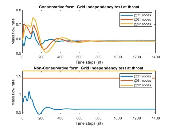
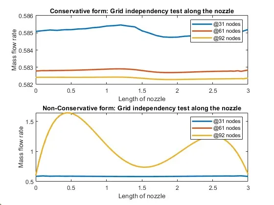
If we look at the throat section and inside the nozzle we can conclude that if we increase the number of points also there is no significant change in the result. The slight changes in these graphs are considerably insignificant.
Just to see the effect of CFL on these mass flow rates I ran a couple more simulations where CFL is 0.1 and 1.2. Here are the results
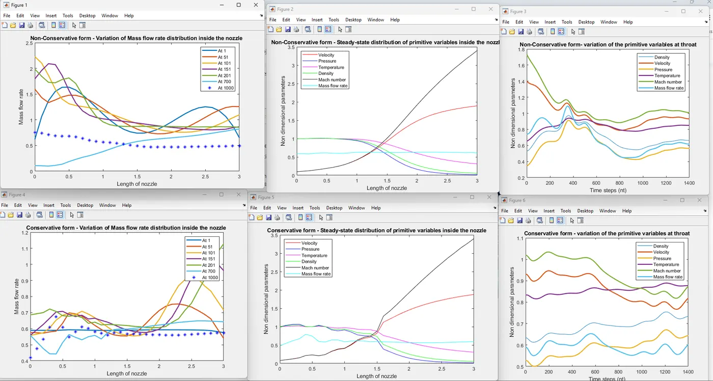
Here we can see all the six graphs in one snippet. the results are a little bit different compared to CFL 0.5 but follow the same trend in mass flow rate and primitive variables.
Let's look at the comparison of mass flow rate at throat and in nozzle
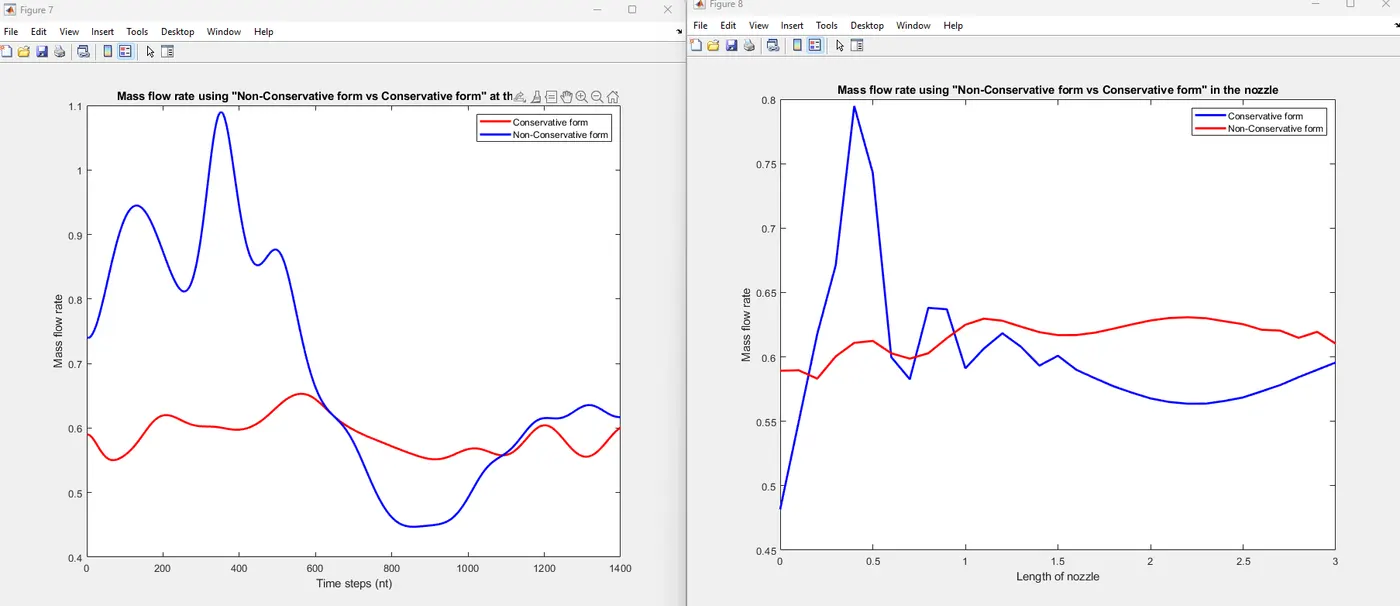
In both at throat and inside the nozzle we can observe the same pattern that the conservation equation and non-conservation equations did not reach the steady state but the conservation form has closer values from one another.
if the CFL is 1.2 how are the results looking lets test?
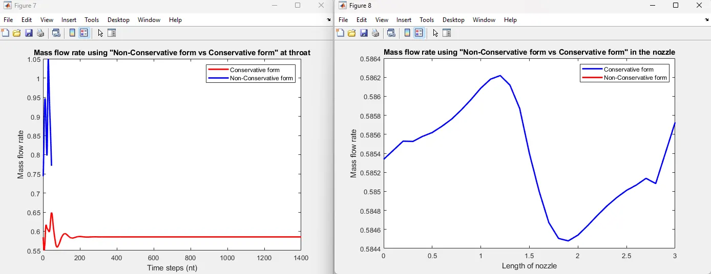
If we look at the comparison of the mass flow rate in the nozzle and at the throat section. The results are starting to blow up after 1.2. So it is recommended to choose a CFL number less than 1.2. to avoid an unstable solution.