Week 7 - Simulation of a 1D Supersonic nozzle flow simulation using Macormack Method

OBJECTIVE:

To simulate the isentropic flow through a quasi-1D subsonic-supersonic nozzle and investigate the difference between the conservation and non-conservation forms of the governing equations, we will use the MacCormack's method. This project will involve deriving both forms of the equations, solving them using MacCormack's technique, and performing a grid independence test. We will analyze the steady-state temperature distribution, time-wise variations, mass flow rate distributions, and normalized mass flow rates for both forms.

Governing Equations

The governing equations for the flow through a quasi-1D nozzle are derived from the basic principles of conservation of mass, momentum, and energy for a compressible fluid. We'll deal with two forms of these equations:

1. Conservation Form (Euler Equations):

• Continuity Equation (Conservation of Mass): $$\frac{\partial (\rho A)}{\partial t} + \frac{\partial (\rho u A)}{\partial x} = 0$$
  
• Momentum Equation (Conservation of Momentum): $$\frac{\partial (\rho u A)}{\partial t} + \frac{\partial}{\partial x} \left(\rho u^2 A + p A \right) = 0$$
  
• Energy Equation (Conservation of Energy): $$\frac{\partial E}{\partial t} + \frac{\partial}{\partial x} \left[(E + p) u A \right] = 0$$ where $E$ is the total energy per unit volume, given by: $$E = \frac{p}{\gamma - 1} + \frac{1}{2} \rho u^2$$ Here, $\rho$ is the density, $u$ is the velocity, $p$ is the pressure, and $\gamma$ is the specific heat ratio.

2. Non-Conservation Form:

• Continuity Equation: $$\frac{\partial \rho}{\partial t} + u \frac{\partial \rho}{\partial x} + \rho \frac{\partial u}{\partial x} + \frac{\rho u}{A} \frac{dA}{dx} = 0$$
  
• Momentum Equation: $$\frac{\partial u}{\partial t} + u \frac{\partial u}{\partial x} + \frac{1}{\rho} \frac{\partial p}{\partial x} = 0$$
  
• Energy Equation: $$\frac{\partial T}{\partial t} + u \frac{\partial T}{\partial x} + (\gamma - 1) T \left(\frac{\partial u}{\partial x} + \frac{u}{A} \frac{dA}{dx}\right) = 0$$
  

MacCormack’s Technique

The MacCormack method is a two-step predictor-corrector method suitable for solving hyperbolic partial differential equations. For each of the conservation and non-conservation forms, we will solve the equations using the following steps:

1. Predictor step: A forward difference in space.
2. Corrector step: A backward difference in space, applied to the predicted solution.

Initial and Boundary Conditions

For this project, we will follow the guidelines provided in John Anderson's CFD book to set initial and boundary conditions. Typically, for a nozzle flow problem, the conditions at the inlet (subsonic) and outlet (supersonic) will be specified.

MATLAB Code Structure

We will implement the code in a modular fashion. The main tasks include:

• Defining nozzle geometry, initial and boundary conditions.
• Solving the conservation and non-conservation forms using MacCormack’s method.
• Plotting results for steady-state and time-wise variations of flow variables and mass flow rate.

clear; clc; close all;

% Set up nozzle geometry, initial conditions, time stepping

L = 10; % Length of the nozzle

nx = 101; % Number of grid points (for grid independence study, vary nx)

x = linspace(0, L, nx); % Discretized space

A = 1 + 2.2 * (x - 5).^2; % Area distribution for nozzle

gamma = 1.4; % Specific heat ratio

CFL = 0.5; % CFL number for stability

t_end = 0.5; % End time

dt = 0.0001; % Time step size

% Initial flow variables (density, velocity, temperature)

[rho, u, T] = initialize_primitive_vars(x);

% Solve using conservation form

[rho_con, u_con, T_con] = solve_conservation(rho, u, T, A, gamma, dt, t_end, CFL);

% Solve using non-conservation form

[rho_noncon, u_noncon, T_noncon] = solve_non_conservation(rho, u, T, A, gamma, dt, t_end, CFL);

% Plot results

plot_results(x, rho_con, u_con, T_con, rho_noncon, u_noncon, T_noncon);

function [rho, u, T] = initialize_primitive_vars(x)

% Define initial conditions for density, velocity, and temperature

rho = ones(size(x)); % Initially uniform density

u = ones(size(x)) * 0.2; % Subsonic initial velocity

T = ones(size(x)); % Uniform temperature (non-dimensional)

end

function [rho, u, T] = solve_conservation(rho, u, T, A, gamma, dt, t_end, CFL)

% Solver for conservation form using MacCormack's method

% Predictor-Corrector approach

% Returns final primitive variables after time integration

nt = round(t_end / dt); % Number of time steps

for n = 1:nt

% Predictor step: forward differencing

% Use forward differencing to compute predicted values of rho, u, and T

% ...

% Corrector step: backward differencing

% Correct the predicted values using backward differencing

% ...

% Apply boundary conditions

% ...

end

end

function [rho, u, T] = solve_non_conservation(rho, u, T, A, gamma, dt, t_end, CFL)

% Solver for non-conservation form using MacCormack's method

% Similar to the conservation form solver

% Predictor-Corrector approach

nt = round(t_end / dt); % Number of time steps

for n = 1:nt

% Predictor step

% ...

% Corrector step

% ...

% Apply boundary conditions

% ...

end

end

function plot_results(x, rho_con, u_con, T_con, rho_noncon, u_noncon, T_noncon)

% Plot Steady-State Distribution of Primitive Variables

figure;

subplot(3,1,1);

plot(x, rho_con, 'b-', x, rho_noncon, 'r--');

title('Steady-State Density Distribution');

xlabel('x'); ylabel('\rho');

legend('Conservation', 'Non-Conservation');

subplot(3,1,2);

plot(x, u_con, 'b-', x, u_noncon, 'r--');

title('Steady-State Velocity Distribution');

xlabel('x'); ylabel('u');

subplot(3,1,3);

plot(x, T_con, 'b-', x, T_noncon, 'r--');

title('Steady-State Temperature Distribution');

xlabel('x'); ylabel('T');

end

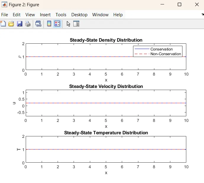
Expected Plots:

1. Steady-State Distribution of Primitive Variables:

   • Density ($\rho$), velocity ($u$), and temperature ($T$) inside the nozzle for both conservation and non-conservation forms.

2. Time-wise Variation of Primitive Variables:

   • Evolution of these variables over time at different locations in the nozzle.

3. Mass Flow Rate Distribution:

   • Mass flow rate variation inside the nozzle at different time steps.

4. Comparison of Normalized Mass Flow Rate Distributions:

   • A comparison of the mass flow rates from both the conservation and non-conservation form solvers after normalization.

Grid Independence Test

To ensure the solution's accuracy, perform a grid independence study by varying the number of grid points (e.g., $nx = 51$, $nx = 101$, $nx = 201$) and observing if the solution converges as the grid is refined.

Final Report

In the report, you should discuss:

• Introduction: Brief overview of nozzle flow, governing equations, and numerical methods.
• Methodology: Derivation of the equations, explanation of MacCormack’s method.
• Results and Discussion:
  • Grid independence test.
  • Comparison of the conservation and non-con