Challenge

Week 7 - Simulation of a 1D Supersonic nozzle flow simulation using Macormack Method

AAkash Shenvi23 Aug 2023

Aim :- Simulation of a 1D Super-sonic nozzle flow simulation using Macormack Method

Objective :- To simulate 1D Supersonic nozzle flow using McCormack Technique by implementing conservative and non conservative form of governing equations using MATLAB program.

Problem Statement :-

Determine the steady-state temperature distribution for the flow-field variables & investigate the difference between the two forms of governing equations by comparing their solutions.

1. Steady-state distribution of primitive variables inside the nozzle
2. Time-wise variation of the primitive variables
3. Variation of Mass flow rate distribution inside the nozzle at different time steps during the time-marching process
4. Comparison of Normalized mass flow rate distributions of both forms

Theory Introduction :-

CD Nozzle :-

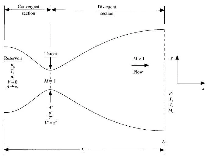
Convergent Divergent Nozzle also known as De-Laval nozzles are devices that are used to accelerate fluids to very high speeds. CD nozzles are commonly used in propulsion system of supersonic aircraft, spacecraft & in supersonic wind tunnels. A CD nozzle is shaped such that the cross sectional area varies with the axial distance along the length of the nozzle. The shape of the CD nozzle resembles that of an hour glass. There is a minimum area section called the throat, which is proceeded by a converging section & succeeded by a diverging section.

Let us consider a CD nozzle. The inlet station feeds from a large reservoir operating at the stagnation condition of P0, rho0 & T0. When the ambient or back pressure at the exit of the nozzle is small enough, a supersonic flow will be established. In the converging section the flow will always be subsonic. This sonic flow enters the diverging section where it is further accelerated.

Normally we consider the flow properties which vary in both x & y directions, but here in this project we have assumed the flow to vary only along the x axis. So the flow under the assumption is called as Quasi One dimensional flow.

Macormack Method :-

Some of the methods that are available for linear equation are really not well suited for non-linear equation. Multi step methods are methods that uses Finite difference schemes which uses split time levels. These are well suited for Non-Linear Hyperbolic problems. They are also called as Predictor corrector method.

One of those multi step method is Macormack method. It is also a two-step method. Step one uses forward difference scheme & the temporary value for the solution is predicted. Step two uses backward difference scheme & the last step is to take the average of both these steps. This is a second order method well suited for solving non-linear equations in both space & time.

Predictor Method :-

In predictor method, the spacial derivatives on the right hand side are replaced by forward difference scheme.

Hence consider continuity equation in one dimension

i,j is the space grid

t- is the time, dt is the time step, dx is the grid size.

Corrector Method :-

In corrector method, the spacial derivatives on the right hand side are replaced by backward difference scheme.

i,j is the space grid

t- is the time, dt is the time step, dx is the grid size.

Governing Equation :-

Governing equations are of two forms:

1) Non Conservative form :-

The Non Conservative form of equations are no different from conservative equation mathematically. But physically Non Conservative form is derived based on finite control volume moving with fluid.

The equations are expressed by non-dimensional variables.

2) Conservative form :-

The Conservative form of equations are no different from Non Conservative equation mathematically. But physically Conservative form is derived based on finite control volume fixed in space.

The equations are expressed in integral or differential forms.

Main Code :-

Non-Conservative form :-

%Week 7 - Simulation of a 1D Super-sonic nozzle flow simulation using McCormack Method:
%Non-Conservative Form
clear all
close all
clc

%Inputs
n=31;%Assigning Grid points
x=linspace(0,3,n);%Length
dx=x(2)-x(1);
gamma=1.4;

%calculating initial profiles
rho=1-0.3146*x;% Density
t=1-0.2314*x;%t=temperature
v=(0.1+1.09*x).*t.^0.5;%velocity

%Area
a=1+2.2*(x-1.5).^2;

%timesteps
nt=1400;
dt=0.04;
throat=round(n/2);
cfl=max((v+sqrt(t))*dt/dx);

%outer time loop
for k=1:nt

    rho_old=rho;
    v_old=v;
    t_old=t;

    %Predictor method
    for j=2:n-1 %for inner nodes

        dvdx=(v(j+1)-v(j))/dx;
        drhodx=(rho(j+1)-rho(j))/dx;
        dtdx=(t(j+1)-t(j))/dx;
        dlogadx=(log(a(j+1))-log(a(j)))/dx;

        %continuity equation
        drhodt_p(j)=-rho(j)*dvdx-rho(j)*v(j)*dlogadx-v(j)*drhodx;

        %momentum equation
        dvdt_p(j)=-v(j)*dvdx-(1/gamma)*(dtdx+(t(j)/rho(j))*drhodx);

        %energy equation
        dtdt_p(j)=-v(j)*dtdx-(gamma-1)*t(j)*(dvdx+v(j)*dlogadx);

        %solution update
        rho(j)=rho(j)+drhodt_p(j)*dt;
        v(j)=v(j)+dvdt_p(j)*dt;
        t(j)=t(j)+dtdt_p(j)*dt;

    end

    %corrector method
    for j=2:n-1 %for inner nodes

        dvdx=(v(j)-v(j-1))/dx;
        drhodx=(rho(j)-rho(j-1))/dx;
        dtdx=(t(j)-t(j-1))/dx;
        dlogadx=(log(a(j))-log(a(j-1)))/dx;

        %continuity equation
        drhodt_c(j)=-rho(j)*dvdx-rho(j)*v(j)*dlogadx-v(j)*drhodx;

        %momentum equation
        dvdt_c(j)=-v(j)*dvdx-(1/gamma)*(dtdx+(t(j)/rho(j))*drhodx);

        %energy equation
        dtdt_c(j)=-v(j)*dtdx-(gamma-1)*t(j)*(dvdx+v(j)*dlogadx);
      
     end

    %compute the average time derivative
    drhodt=0.5*(drhodt_p+drhodt_c);
    dvdt=0.5*(dvdt_p+dvdt_c);
    dtdt=0.5*(dtdt_p+dtdt_c);

    %final solution update
    for i=2:n-1
       rho(i)=rho_old(i)+drhodt(i)*dt;
       v(i)=v_old(i)+dvdt(i)*dt;
       t(i)=t_old(i)+dtdt(i)*dt;
    end

    %Apply Boundary Condition
    %Inlet Boundary Condition
    v(1)=2*v(2)-v(3);

    %outlet
    v(n)=2*v(n-1)-v(n-2);
    rho(n)=2*rho(n-1)-rho(n-2);
    t(n)=2*t(n-1)-t(n-2);

    %Pressure
    p=rho.*t;

    %Mach number
    M=v./sqrt(t); %a=sqrt(gamma*Gas const*Temperature)==>in which we have considered gamma and gas constant as 1.

    %Mass flow rate
    m=rho.*a.*v;
    
    %Finding the values of Density,Velocity,Temperature,Pressure and Mach
    %Number at the throat point
    rho_throat(k)=rho(throat);
    v_throat(k)=v(throat);
    t_throat(k)=t(throat);
    p_throat(k)=p(throat);
    M_throat(k)=M(throat);

    figure(1)
    hold on
    if k==1
        plot(x,m)
    end
    if k==50
        plot(x,m)
    end
    if k==250
        plot(x,m)
    end
    if k==500
        plot(x,m)
    end
    if k==750
        plot(x,m)
    end
    if k==1400
        plot(x,m)
    end

end
xlabel('Nozzle Length')
ylabel('Mass flow rate')
legend('1dt','50dt','250dt','500dt','750dt','1400dt')
title('Variation of mass flow rate at different time steps')

figure(2)
subplot(5,1,1)
plot(x,v)
xlabel('Nozzle Length')
ylabel('Velocity')
title('Steady state primitive variable profiles')
subplot(5,1,2)
plot(x,rho)
xlabel('Nozzle Length')
ylabel('Density')
subplot(5,1,3)
plot(x,t)
xlabel('Nozzle Length')
ylabel('Temperature')
subplot(5,1,4)
plot(x,p)
xlabel('Nozzle Length')
ylabel('Pressure')
subplot(5,1,5)
plot(x,M)
xlabel('Nozzle Length')
ylabel('Mach No')

figure(3)
plot(x,m)
xlabel('Nozzle Length')
ylabel('Mass flow rate')
title('Steady state mass flow rate profiles')

figure(4)
subplot(5,1,1)
plot(v_throat)
xlabel('Time step')
ylabel('Velocity')
title('Transient variation of primitive variables at throat')
subplot(5,1,2)
plot(rho_throat)
xlabel('Time step')
ylabel('Density')
subplot(5,1,3)
plot(t_throat)
xlabel('Time step')
ylabel('Temperature')
subplot(5,1,4)
plot(p_throat)
xlabel('Time step')
ylabel('Pressure')
subplot(5,1,5)
plot(M_throat)
xlabel('Time step')
ylabel('Mach No')

Explanation :-

Input Variables of n,x,dx and gamma are assigned with the values.
Calculation of initial profiles of density, temperature & velocity are asigned.
Formula for finding the area of the nozzle is assigned.
Timesteps values are assigned.
Throat point value & CFL values are computed.
For loop for time loop is assigned with the total number of timesteps.
Copies for the values of density, temperature and velocity are done.
For loop for predictor & corrector methods are assigned individually.
The continuity, momentum & energy equation for the predictor & corrector methods are found by forward & backward differencing schemes respectively.
Solution update is done for the predictor method.
The average time derivation is computed.
Final solution update is done.
Boundary conditions for inlet & outlet are assigned.
The values for the pressure, mach number & mass flow rate are computed.
Required graphs are plotted.

Plots :-

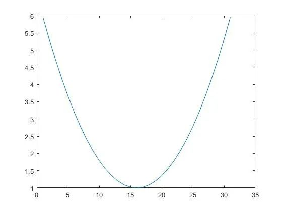
This plot represents the area of the nozzle through the nodes of 31 points.

Non-Dimensional Primitive Variable Profiles(Non-Conservative form) :-

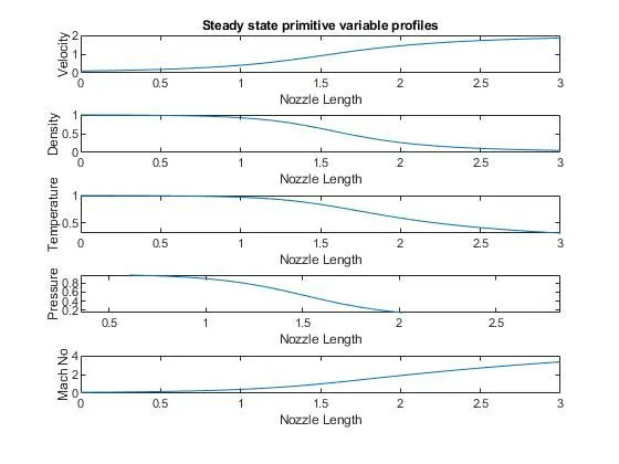
The above mentioned graph shows relation between the length of the nozzle & Velocity, Density, Temperature, Pressure & Mach no.

Mass Flow Rate :-

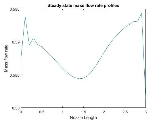
The above graph shows the relation between the length of the nozzle & the mass flow rate acquired.

Non-Dimensional flow variables at throat section :-

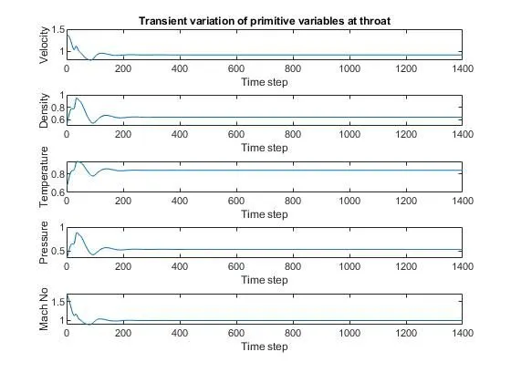
This graph shows the relation between the Time step & Velocity, Density, Temperature, Pressure, Mach no at the throat section.

The throat section point is evaluated by:

round(n/2) command in Matlab code.

Variation of mass flow rate at different time steps :-

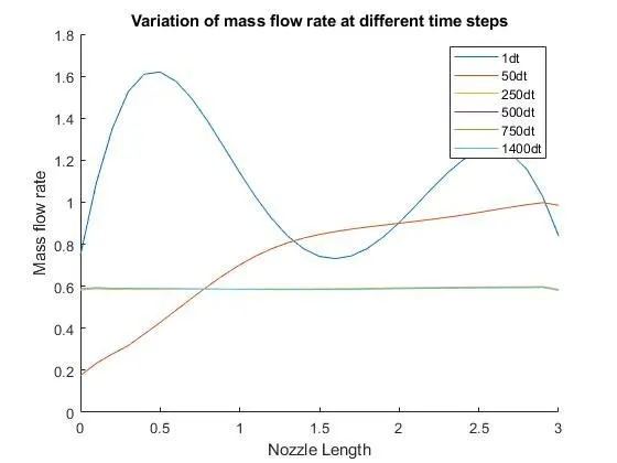
This graph represents the relation between the lenght of the nozzle & the primitive variables calculated at the time steps of 1dt, 50dt,250dt, 500dt, 750dt,1400dt.

Conservative form :-

Main code :-

%Week 7 - Simulation of a 1D Super-sonic nozzle flow simulation using McCormack Method:
%Conservative Form
clear all
close all
clc

%Inputs
n=31;%Assigning Grid points
x=linspace(0,3,n);%Length
dx=x(2)-x(1);
gamma=1.4;

%Initial profiles
for i=1:n 

    if x(i)<=0.5

        rho(i)=1;
        t(i)=1;

    end

    if  x(i)>0.5 && x(i)<=1.5

        rho(i)=1 - 0.366*(x(i)-0.5);
        t(i)=1 - 0.167*(x(i)-0.5);

    end

     if  x(i)>1.5

        rho(i)=0.634-0.3879*(x(i)-1.5);
        t(i)=0.833-0.3507*(x(i)-1.5);

     end

end


%timesteps
nt=1400;
dt=0.0267;
throat=round(n/2);

%Area
a=1+2.2*(x-1.5).^2;
v=0.59./(rho.*a);
U1=rho.*a;
U2=rho.*a.*v;
U3=U1.*(t/(gamma-1)+(gamma/2)*v.^2);
cfl=max((v+sqrt(t))*dt/dx);

%outer time loop
for k=1:nt

    U1_old=U1;
    U2_old=U2;
    U3_old=U3;

    F1=U2;
    F2=U2.^2./U1+ ((gamma-1)/gamma) * (U3- (gamma/2) * (U2.^2./U1));
    F3=gamma*U2.*U3./U1 - 0.5*gamma*(gamma-1) * (U2.^3./U1.^2);

    %Predictor method
    for j=2:n-1 %for inner nodes


        %continuity equation
        dU1dt_p(j)=-(F1(j+1)-F1(j))/dx;

        J2=(1/gamma).*rho(j).*t(j).*((a(j+1)-a(j))/dx);
        %momentum equation
        dU2dt_p(j)=-(F2(j+1)-F2(j))/dx+J2;

        %energy equation
        dU3dt_p(j)=-(F3(j+1)-F3(j))/dx;

        %solution update
        U1(j)=U1(j)+dU1dt_p(j)*dt;
        U2(j)=U2(j)+dU2dt_p(j)*dt;
        U3(j)=U3(j)+dU3dt_p(j)*dt;

    end
    
    %Predictor update
    rho=U1./a;
    t=(gamma-1).*(U3./U1-(gamma/2)*(U2./U1).^2);
    F1=U2;
    F2=U2.^2./U1+ ((gamma-1)/gamma) * (U3- (gamma/2) * (U2.^2./U1));
    F3=gamma*U2.*U3./U1 - 0.5*gamma*(gamma-1) * (U2.^3./U1.^2);


    %corrector method
    for j=2:n-1 %for inner nodes


        %continuity equation
        dU1dt_c(j)=-(F1(j)-F1(j-1))/dx;

        J2=(1/gamma)*rho(j)*t(j)*(a(j)-a(j-1))/dx;
        %momentum equation
        dU2dt_c(j)=-(F2(j)-F2(j-1))/dx+J2;

        %energy equation
        dU3dt_c(j)=-(F3(j)-F3(j-1))/dx;

      
    end

    %compute the average time derivative
    dU1dt=0.5.*(dU1dt_p+dU1dt_c);
    dU2dt=0.5.*(dU2dt_p+dU2dt_c);
    dU3dt=0.5.*(dU3dt_p+dU3dt_c);

    %final solution update
    for l=2:n-1
       U1(l)=U1_old(l)+dU1dt(l)*dt;
       U2(l)=U2_old(l)+dU2dt(l)*dt;
       U3(l)=U3_old(l)+dU3dt(l)*dt;
    end

    %Final Update
    rho=U1./a;
    t=(gamma-1)*(U3./U1-(gamma/2)*(U2./U1).^2);
    v=U2./U1;


    %Apply Boundary Condition
    %Inlet Boundary Condition
    U1(1)=a(1);
    U2(1)=2*U2(2)-U2(3);
    U3(1)=U1(1)*(t(1)/(gamma-1)+0.5*gamma*v(1)^2);

    %outlet
    U1(n)=2*U1(n-1)-U1(n-2);
    U2(n)=2*U2(n-1)-U2(n-2);
    U3(n)=2*U3(n-1)-U3(n-2);

    %Pressure
    p=rho.*t;

    %Mach number
    M=v./sqrt(t); %a=sqrt(gamma*Gas const*Temperature)==>in which we have considered gamma and gas constant as 1.

    %Mass flow rate
    m=rho.*a.*v;
    
    %Finding the values of Density,Velocity,Temperature,Pressure and Mach
    %Number at the throat point
    rho_throat(k)=rho(throat);
    v_throat(k)=v(throat);
    t_throat(k)=t(throat);
    p_throat(k)=p(throat);
    M_throat(k)=M(throat);

    figure(1)
    hold on
    if k==1
        plot(x,m)
    end
    if k==50
        plot(x,m)
    end
    if k==250
        plot(x,m)
    end
    if k==500
        plot(x,m)
    end
    if k==750
        plot(x,m)
    end
    if k==1400
        plot(x,m)
    end

end
xlabel('Nozzle Length')
ylabel('Mass flow rate')
legend('1dt','50dt','250dt','500dt','750dt','1400dt')
title('Variation of mass flow rate at different time steps')

figure(2)
subplot(5,1,1)
plot(x,v)
xlabel('Nozzle Length')
ylabel('Velocity')
title('Steady state primitive variable profiles')
subplot(5,1,2)
plot(x,rho)
xlabel('Nozzle Length')
ylabel('Density')
subplot(5,1,3)
plot(x,t)
xlabel('Nozzle Length')
ylabel('Temperature')
subplot(5,1,4)
plot(x,p)
xlabel('Nozzle Length')
ylabel('Pressure')
subplot(5,1,5)
plot(x,M)
xlabel('Nozzle Length')
ylabel('Mach No')

figure(3)
plot(x,m)
xlabel('Nozzle Length')
ylabel('Mass flow rate')
title('Steady state mass flow rate profiles')

figure(4)
subplot(5,1,1)
plot(v_throat)
xlabel('Time step')
ylabel('Velocity')
title('Transient variation of primitive variables at throat')
subplot(5,1,2)
plot(rho_throat)
xlabel('Time step')
ylabel('Density')
subplot(5,1,3)
plot(t_throat)
xlabel('Time step')
ylabel('Temperature')
subplot(5,1,4)
plot(p_throat)
xlabel('Time step')
ylabel('Pressure')
subplot(5,1,5)
plot(M_throat)
xlabel('Time step')
ylabel('Mach No')

Plots :-

Steady State Primitive Variables in Conservative form :-

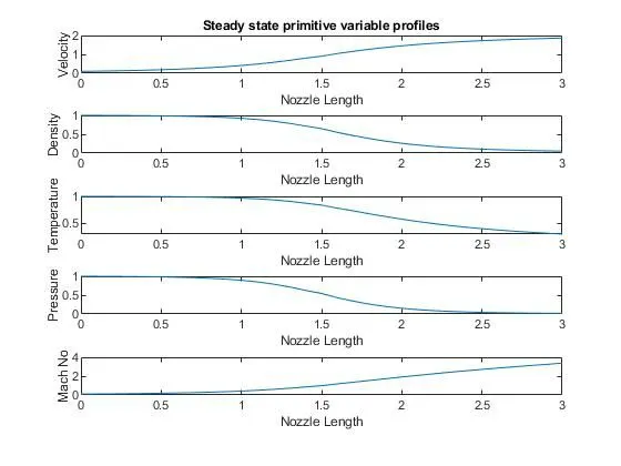
The above plots are almost the same when compared to the analytical solution referred from Anderson Textbook. We can observe from the above graphs that while the Velocity & Mach Number increase from inlet to outlet, it comes at an expense of a drop in pressure, density & temperature along the same path of the inlet to outlet. From Bernoulli's equation we know that in the case of horizontal flow, an increase in velocity must be accompanied by a decrease in pressure because of conservation of energy. The energy required to increase the fluid's velocity comes at an expense of static pressure energy.

Variation of Mass Flow Rate distributed inside the nozzle at different time steps during the time marching process-Conservative form :-

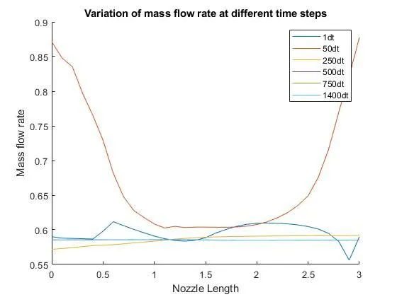
This graph represents the relation between the lenght of the nozzle & the primitive variables calculated at the time steps of 1dt, 50dt,250dt, 500dt, 750dt,1400dt.

Time wise variation of various Primitive Variables at the throat using the Conservative method :-

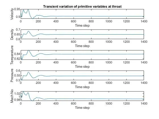
From above plot we can infer that the time wise variation of non-dimensional flow field variables at the throat in conservative form attaining the steady state. We can also observe that the oscillations are reduced to a steady state eventually. Here we can predict that almost 300 timesteps have been taken for the conservative form to attain steady state.

Grid Dependence Test :-

Here by varying the grid points we can check the accuracy of the result. So as we increase the number of grid points, the accuracy of the result will also be increased. On increasing the grid points it is observed that it is reaching close to the actual /analytical solution.

Conclusion :-

It is observed that there is good accuracy on increasing the grid points.

The mass flow rate is better in conservative form as it reaches close to the analytical solution when compared to the non-conservative form solution.

For mass flow rate in non-conservative form, the solution needs much higher time steps as at lower time steps its still having the disturbances at inflow & outflow.

As we know non-conservative form includes primitive variables & conservative form includes flux variables, both tend to give the better outputs for their variables at higher time steps with a very small difference between them.

Week 7 - Simulation of a 1D Supersonic nozzle flow simulation using Macormack Method

Ship work like this
in your own course.

Talk to a career counsellor

Ship work like thisin your own course.

Talk to a career counsellor

Ship work like this
in your own course.