Rankine cycle Simulator

clear all
close all
clc

% Rankine Cycle Simulator
fprintf('Rankine Cyclen')
fprintf('1-2 is Isentropic Expansion in Turbinen')
fprintf('2-3 is constant pressure heat removaln')
fprintf('3-4 is Isentropic compression in pump n')
fprintf('4-1 is constant pressure heat addition in boilern')

% Entering the input data for calculation of state points
p1 = 30;
T1 = 400;
p2 = 0.05;

% Taking data from Xsteam file for state point 1
h1 = XSteam('h_pT',p1,T1);
s1 = XSteam('s_pT',p1,T1);

% Taking data from Xsteam file for state point 2
s2 = s1;
sf2 = XSteam('sL_p',p2);
sg2 = XSteam('sV_p',p2);
x2 = (s2-sf2)/(sg2-sf2);
hf2 = XSteam('hL_p',p2);
hg2 = XSteam('hV_p',p2);
h2 = hf2 + (x2*(hg2-hf2));

% Taking data from Xsteam file for state point 3
p3 = p2;
s3 = XSteam('sL_p',p3);
h3 = XSteam('hL_p',p3);

% Taking data from Xsteam file for state point 4
s4 = s3;
p4 = p1;

% Work done in turbine for rankine cycle
W_T = h1-h2;

% Work done required for pump
v3 = XSteam('vL_p',p3);
W_P = v3*(p4-p3)*100;
h4 = h3 - W_P;

% Net work done for Rankine Cycle
W_net = W_T - W_P;

% Heat addition to system
Q_in = h1-h4;

% Heat rejection from system
Q_out = h2-h3;

% Thermal efficiency
T_eff = (W_net/Q_in)*100;

% Specific Steam Consumption = (Mass flow rate / net work done)
Sp_S = (3600/W_net);

% Calculation of Temperature at all state point 2,3 & 4
T3 = XSteam('Tsat_p',p3);
T2 = T3;
Cp4 = XSteam('Cp_ps',p4,s4);
Cv4 = XSteam('Cv_ps',p4,s4);
k = Cp4/Cv4;
T4 = T3/((p3/p4)^((k-1)/k));

% Calculation of other constant
T6 = XSteam('Tsat_p', p1);
s5 = XSteam('sL_p', p1);
s6 = XSteam('sV_p', p1);
h5 = XSteam('hL_p', p1);
h6 = XSteam('hV_p', p1);
T5 = T6;

% Plotting for Saturation line
T = linspace(1,560,1000);
for i = 1:length(T)
sf(i) = XSteam('sL_T',T(i));
sg(i) = XSteam('sV_T',T(i));
hf(i) = XSteam('hL_T',T(i));
hg(i) = XSteam('hV_T',T(i));
end

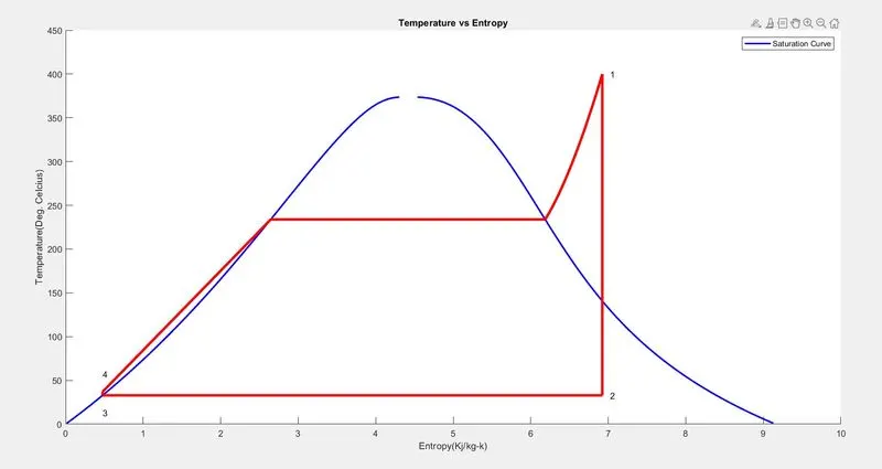
% Plotting T-S Diagram for Rankine Cycle
figure(1)
hold on
plot(sf,T,'color','b','LineWidth',2)
plot(sg,T,'color','b','LineWidth',2)
plot([s1 s2],[T1 T2],'Color','r','linewidth',3)
plot([s2 s3],[T2 T3],'Color','r','linewidth',3)
plot([s3 s4],[T3 T4],'Color','r','linewidth',3)
plot([s4 s5],[T4 T5],'Color','r','linewidth',3)
plot([s5 s6],[T5 T6],'Color','r','linewidth',3)
s_1 = linspace(s6,s1,1000);
for j = 1:length(s_1)
Tc(j) = XSteam('T_ps',p1,s_1(j));
end
plot(s_1,Tc,'Color','r','LineWidth',3)
text(s1+0.1, T1, '1')
text(s2+0.1, T2, '2')
text(s3, T3-20, '3')
text(s4, T4+20, '4')
title('Temperature vs Entropy')
xlabel('Entropy(Kj/kg-k)')
ylabel('Temperature(Deg. Celcius)')
legend('Saturation Curve')

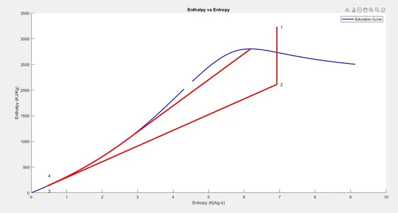
% Plotting H-S Diagram for Rankine cycle
figure(2)
hold on
plot(sf,hf,'color','b','linewidth',2)
plot(sg,hg,'color','b','linewidth',2)
plot([s1 s2],[h1 h2],'Color','r','linewidth',3)
plot([s2 s3],[h2 h3],'Color','r','linewidth',3)
plot([s3 s4],[h3 h4],'Color','r','linewidth',3)
hc = linspace(h4,h5,100);
for k = 1:length(hc)
s_c(k) = XSteam('s_ph',p1,hc(k));
end
plot(s_c,hc,'Color','r','linewidth',3)
plot([s5 s6],[h5 h6],'Color','r','linewidth',3)
for l = 1:length(s_1)
h_c(1) = XSteam('h_ps',p1,s_1(1));
end
plot(s_1,h_c,'Color','r','linewidth',3)
text(s1+0.1,h1,'1')
text(s2+0.1,h2,'2')
text(s3,h3-100,'3')
text(s4,h4+200,'4')
title('Enthalpy vs Entropy')
xlabel('Entropy (Kj/kg-k)')
ylabel('Enthalpy (KJ/Kg)')
legend('Saturation Curve')

% Displaying Results
disp('Results of Rankine cycle')
fprintf('At state point 1ttttt')
fprintf('At state point 2n')
fprintf('P1 = %10f in Bartttt',p1);
fprintf('P2 = %10f in Barn',p2);
fprintf('T1 = %11f in Deg.Celciustt',T1);
fprintf('T2 = %11f in Deg.Celciusn',T2);
fprintf('H1 = %12f in KJ/Kgttt',h1);
fprintf('H2 = %12f in KJ/Kgn',h2);
fprintf('S1 = %9f in KJ/Kg-kttt',s1);
fprintf('S2 = %9f in KJ/Kg-kn',s2);
fprintf('n')
fprintf('At state point 3ttttt')
fprintf('At state point 4n')
fprintf('P3 = %10f in Bartttt',p3);
fprintf('P4 = %10f in Barn',p4);
fprintf('T3 = %11f in Deg.Celciustt',T3);
fprintf('T4 = %11f in Deg.Celciusn',T4);
fprintf('H3 = %12f in KJ/Kgttt',h3);
fprintf('H4 = %12f in KJ/Kgn',h4);
fprintf('S3 = %9f in KJ/Kg-kttt',s3);
fprintf('S4 = %9f in KJ/Kg-kn',s4);
fprintf('n')
fprintf('Turbine Work Done = %14f in KJ/Kgn',W_T)
fprintf('Pump Work Done = %15f in KJ/Kgn',W_P)
fprintf('Net Work Done = %17 in KJ/Kgn',W_net)
fprintf('Thermal Efficiency = %13f in percentn',T_eff)
fprintf('Sp. Steam Consumption = %f in KJ/Kwn',Sp_S)

Code Explanation

-> Creation of Rankine cycle simulator starts with some input values which are required for calculation of other state points.

-> Inputs such as Inlet Pressure of turbine, temperature at turbine inlet & pressure at condenser are mentioned

-> Then I used XSteam Function File

-> From that I got values of enthalpy & entropy at state point 1

-> Term sg & sf are referred to saturated liquid & saturated vapour

-> Similarly other points are taken from XSteam file to calculate other necessary parameters

-> Then plotting is done respectively for T-s & H-s graph

Errors faces & steps taken to overcome them are as follows

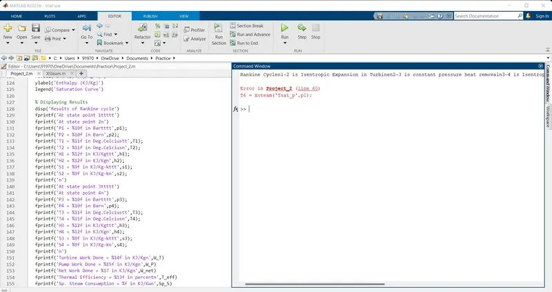
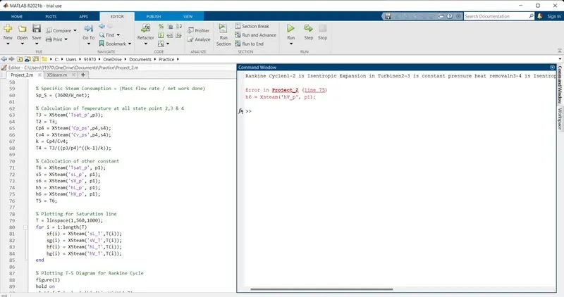
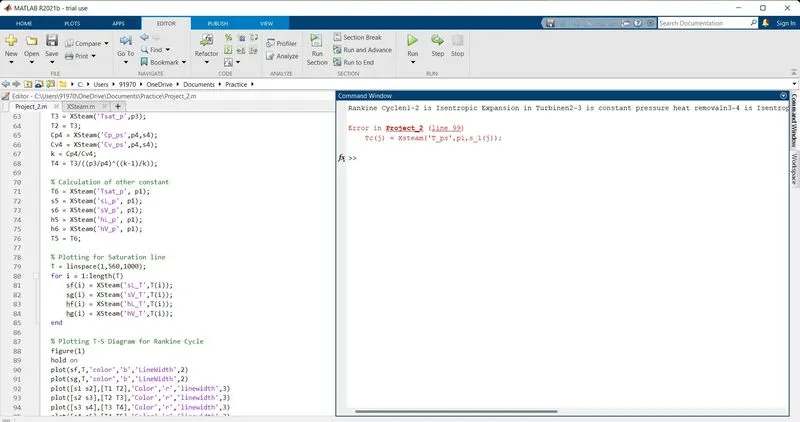
Most common mistakes I made were typing errors where I wrote somewhere capital alphabets or else forgot some coma or brackets which caused the errors but after rectifying them program solved.

Screenshots of errors