Week 7 - Simulation of a 1D Supersonic nozzle flow simulation using Macormack Method
Isentropic flow through a quasi 1D subsonic-supersonic nozzle
- The flow at the inlet to the nozzle tends to be large (A→∞), as the inlet flow is considered to be from reservoir which is large in area.
- And hence the velocity is very small (V→0).
- The Stagnation values of pressure and temperature be Po and To respectively.
- The flow expands isentropically to supersonic speeds at the nozzle exit, where the exit pressure,temperature are represented with subscript e.
- The flow is locally subsonic in the convergent section of the nozzle,sonic at the throat (minimum area) ,and supersonic at the divergent section .
- The sonic flow (M=1) at the throat means the local velocity at this section is equal to the local speed of the sound, and are represented with *.
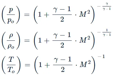
Then,
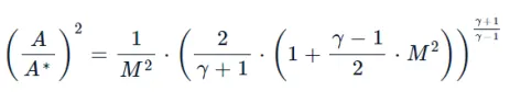
where γ is the ratio of specific heat. (For air γ =1.4)
Mach number:
Mach number is the ratio of flow velocity past a boundary to the local speed of sound.
M = u/c
where:
M is the local Mach number,
u is the local flow velocity, and
c is the speed of sound in the medium.
Mach number in a subsonic compressible flow is derived from Bernoullis equation for M < 1:
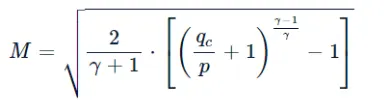
and the speed of sound varies with temperature as follows:
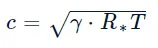
where qc is impact pressure
p is the static pressure.
R∗is the specific gas constant.
MacCormack method:
MacCormack method is a widely used discretization scheme in CFD.
MacCormack's method is an explicit method, provides second order accuracy without the involvement of second order derivative thus reducing the complexity of the calculation.
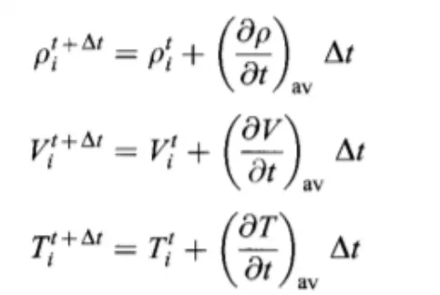
According to this method the value of variable at grid point i,j at time t+dt is given as follows:
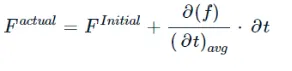
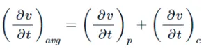
The average time derivative is the half of sum of predictor and corrector values.
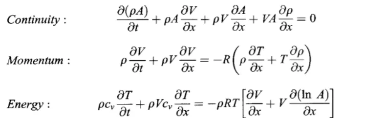
Governing equations:
The super sonic flow through nozzle is governed by Navier stokes equations.
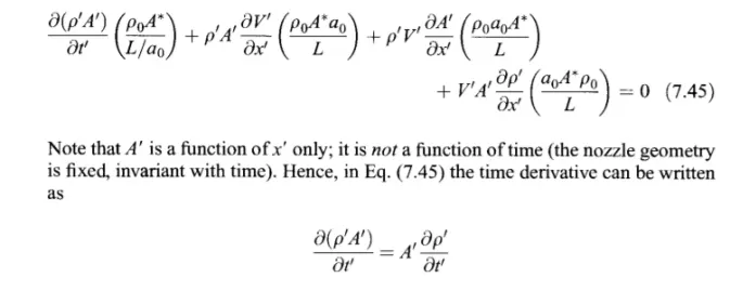
Continuity equation:

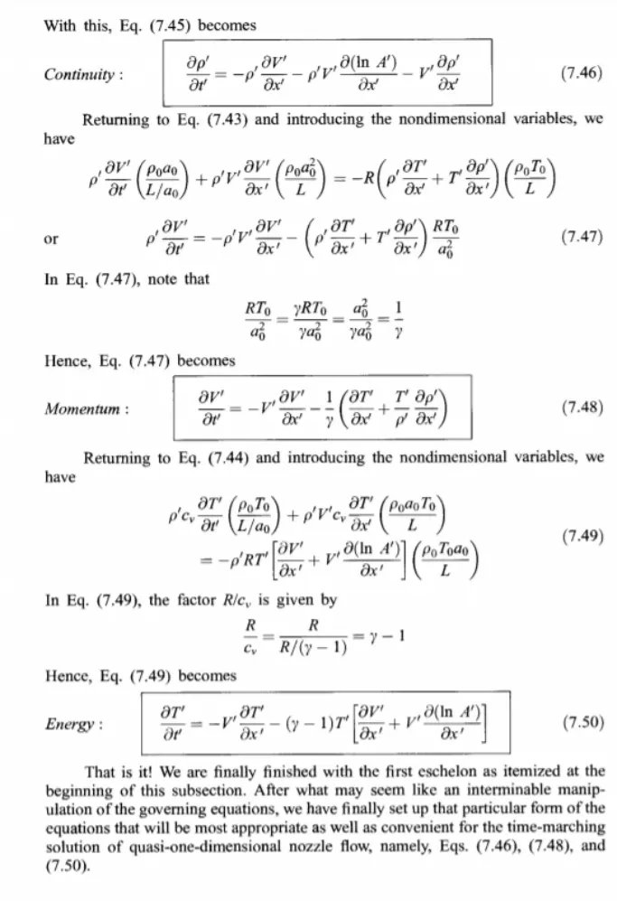
Momentum equation:

Energy equation:

These equation are derived from
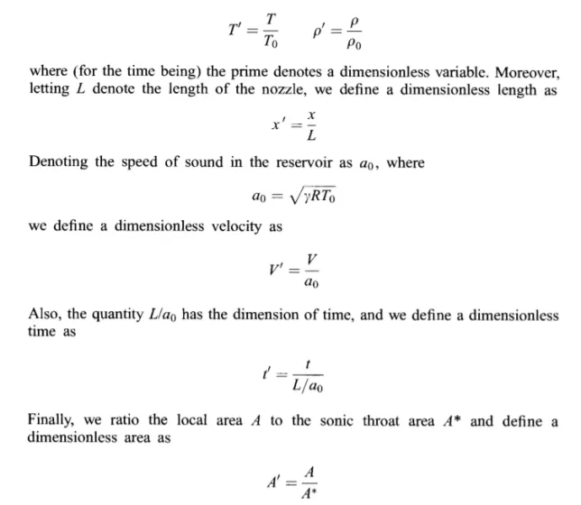
The non dimensional temperature and density respectively as follows:
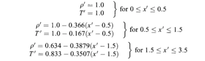
Defining the initial condition :
- The shape of nozzle, A=A(x) is specified and held fixed, independent of time.
- Considering parabolic area distribution

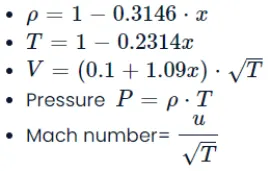
- The density, temperature and velocity is given by
Predictor step:
In this step, we will discretize using forward difference equation.
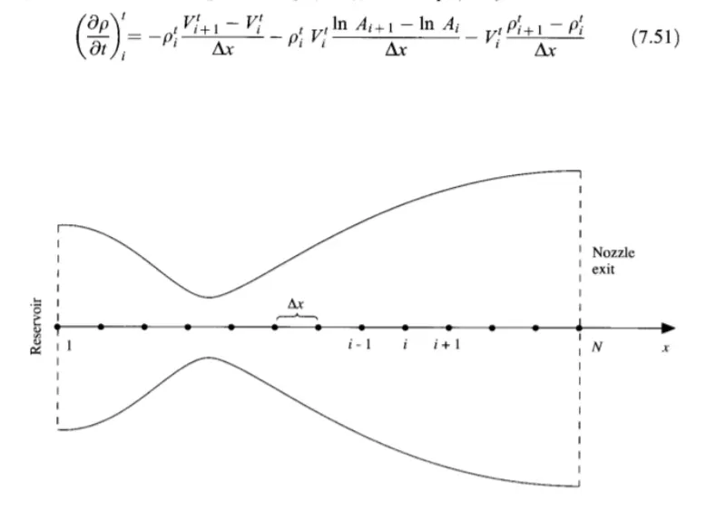
- The length of the nozzle is didvided into number of points along the axis.
- The characteristics of the flow changes from subsonic to super sonic from right to left .
- The distance between the two grid points is dx.
- Smaller the mesh size the error also decreases.
Applying the MacCormach technique to solve the the conservative and non conservative forms of governing equations.
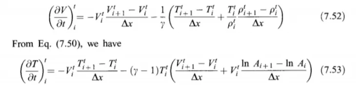
The predicted equation are as follows:
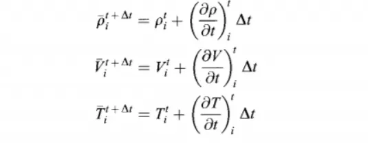
In these equations ρti,Vti and Tti are the known values at time t.
Corrector method:
Applying the backward differencing scheme
Continuity equation
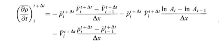
Momentum equation

Energy equation
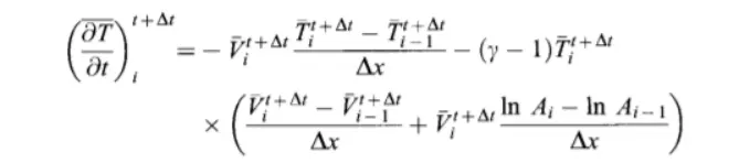
Averaging the sum of corrector and predictor value
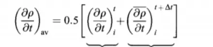
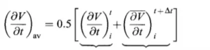

The corrected values at time t+ Δt are:
Calculation of time step:
dt = C * dx / u+a
where C is the courant number
u is the local velocity
a is the local speed of sound
Boundary condtions at subsonic section
By using linear extrapolation
V1= 2 * V2−V3
Density and Temperature at point 1 is held fixed.

Supersonic outflow boundary conditions:
VN = 2*VN−1−VN−2
ρN = 2*ρN−1−ρN−2
TN = 2*TN−1−TN−2
Conservative form
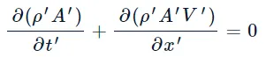
Continuity Equation:
Momentum equation

Energy equation

These are the non dimensional conservative form of the continuity,momentum and energy equations for quasi 1-dimensional flow.
Let the elements of the solution vector U, flux vector F and the source term J as follows
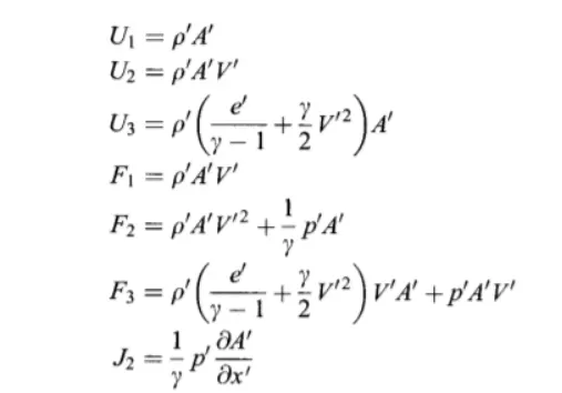
From the above equations we can write that
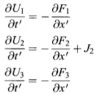
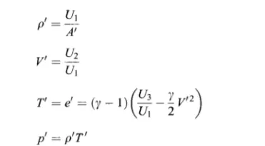
To obtain the primitive variables we must decode the elements U1,U2,U3 as follows. From the definition of U1,U2 and U3 given above we have
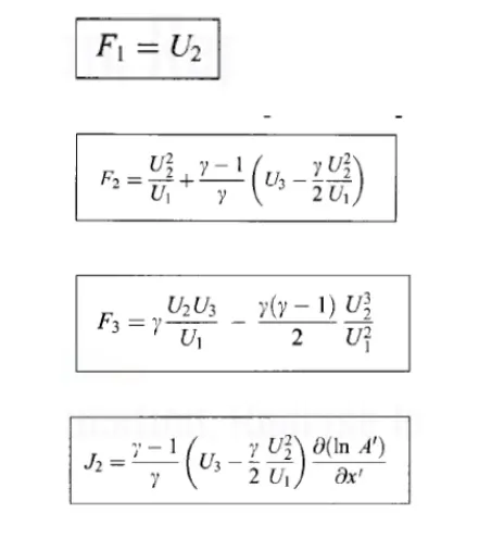
Expressing the flux and source term in form of solution vectors
Applying the boundary conditions @ Inlet
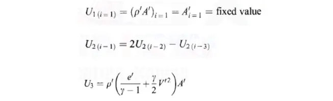
Outlet boundary condition:
The flow properties at the downstream, supersonic outflow boundary can be obtained by linear extrapolation from the two adjacent internal points.
If N denotes the grid point at the outflow boundary ,then:
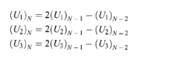
The values of F1,F2 and F3 at grid point i=N are obtained from the values of U1,U2 and U3 at point i=N using the equations.
Initial conditions:
Matlab code:
close all
clear all
clc

% Inputs
n=31;
x=linspace(0,3,n);
dx=x(2)-x(1);
gamma=1.4;
CFL=0.5;
A=1+2.2*(x-1.5).^2;
trt=((n+1)/2);
nt=1400;


tic;
[V,rho,T,m,M,P,V_t,rho_t,T_t,m_t,M_t,P_t]=non_conservative(trt,x,gamma,dx,A,n,nt,CFL);
non_conservative=toc;

tic
[Vc,rhoc,Tc,cons_mass_flow_throat,Mc,pc,Vc_throat,rho_throat,T_throat,cons_mass_flow,Mc_throat,pc_throat]=conservative(trt,x,gamma,dx,A,n,nt,CFL);
conservative=toc;

%plots
figure(3)
plot(x,m,'linewidth',0.95);
hold on;
plot(x,cons_mass_flow,'*');

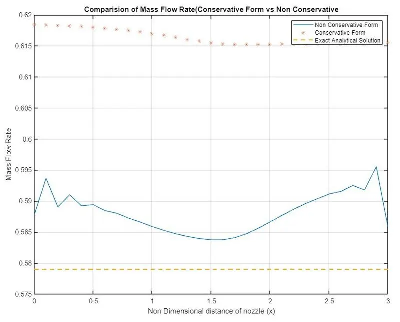
%exact analytical solution rho*A*v=0.579
plot(x,linspace(0.579,0.579,n),'--','linewidth',1.5);
xlabel('Non Dimensional distance of nozzle (x)');
ylabel('Mass Flow Rate');
legend('Non Conservative Form','Conservative Form','Exact Analytical Solution');
title('Comparision of Mass Flow Rate(Conservative Form vs Non Conservative');
grid on ;

figure(4)
plot(x,M,'linewidth',1.5);
hold on
plot(x,Mc,'*','linewidth',0.65,'color','g');
grid on
xlabel('Nozzle(x) Distance');
ylabel('Mach number m');
legend('Non Conservative Form','Conservative Form');
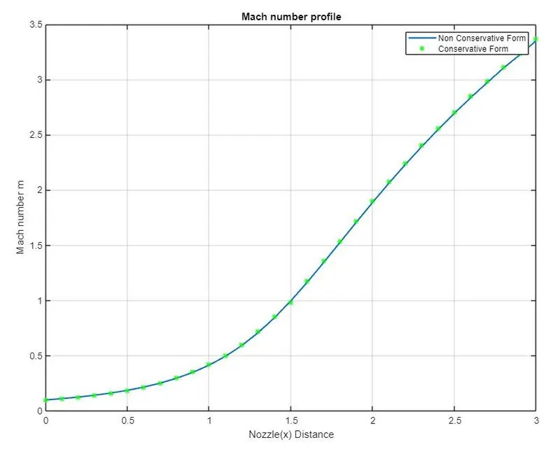
title('Mach number profile');
grid on
figure(5)

plot(x,P,'linewidth',1.25);
hold on
plot(x,pc,'g','linewidth',1.25);
grid on
xlabel('Nozzle(x) Distance');
ylabel('Pressure');
legend('Non Conservative Form','Conservative Form');
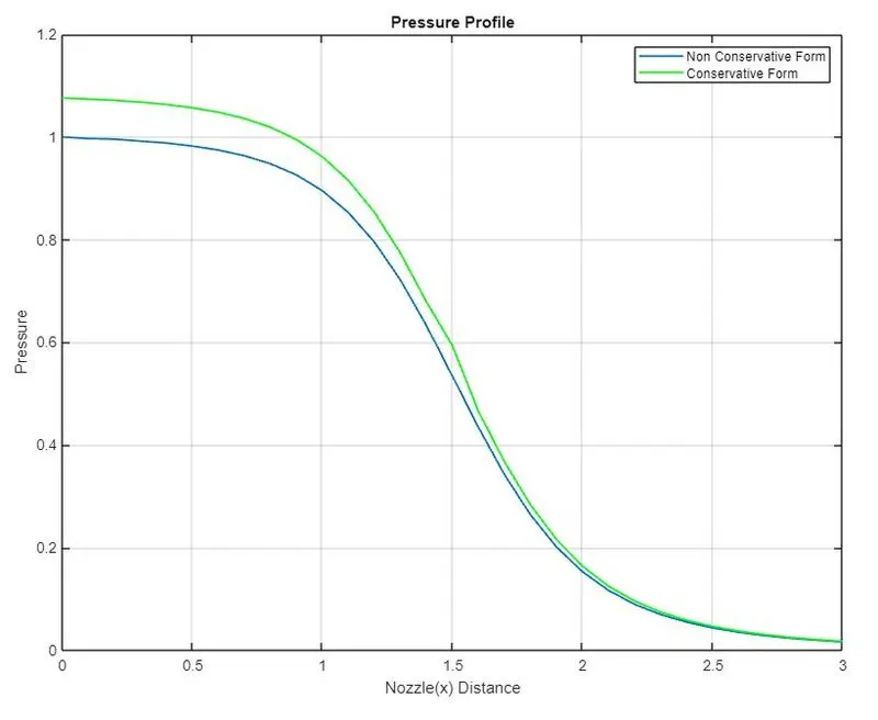
title('Pressure Profile');
grid on

figure(6)
plot(x,rho,'linewidth',1.5)
hold on

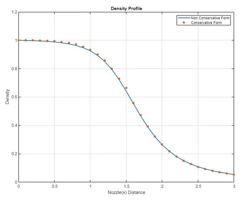
plot(x,rhoc,'*','linewidth',1.25);
grid on
xlabel('Nozzle(x) Distance');
ylabel('Density');
legend('Non Conservative Form','Conservative Form');
title('Density Profile');
grid on
figure(7)

plot(x,T,'linewidth',1.5);
hold on
plot(x,Tc,'*','linewidth',0.65,'color','g');
grid on
xlabel('Nozzle(x) Distance ');
ylabel('Temperature');
legend('Non Conservative Form','Conservative Form');
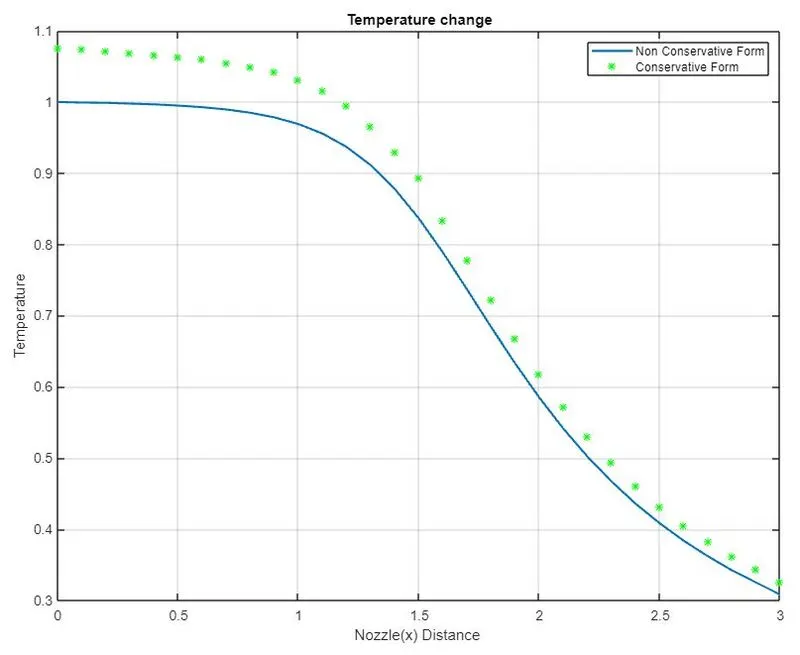
title('Temperature change');

figure(8)
plot(x,V,'linewidth',1.0);
hold on ;
plot(x,Vc,'*','linewidth',0.65,'color','g');
grid on
xlabel('Nozzle(x) Distance');
ylabel('velocity');
legend('Non Conservative Form','Conservative Form');
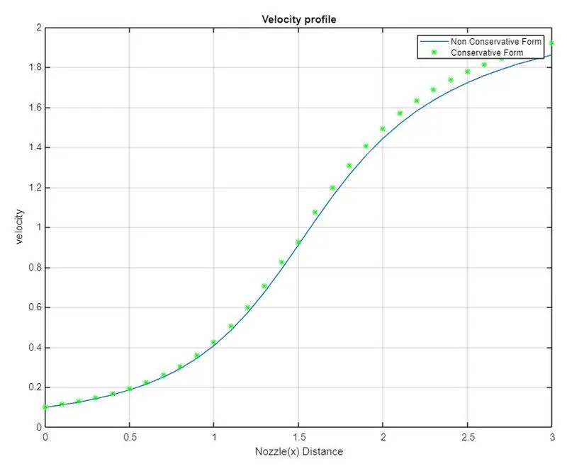
title('Velocity profile');

grid on

figure(9)

plot(1:nt,rho_throat,'linewidth',1.5);
hold on
plot(1:nt,rho_t,'c','linewidth',1.65);
grid on
ylabel('density');
legend('Conservative Form','Non Conservative Form');
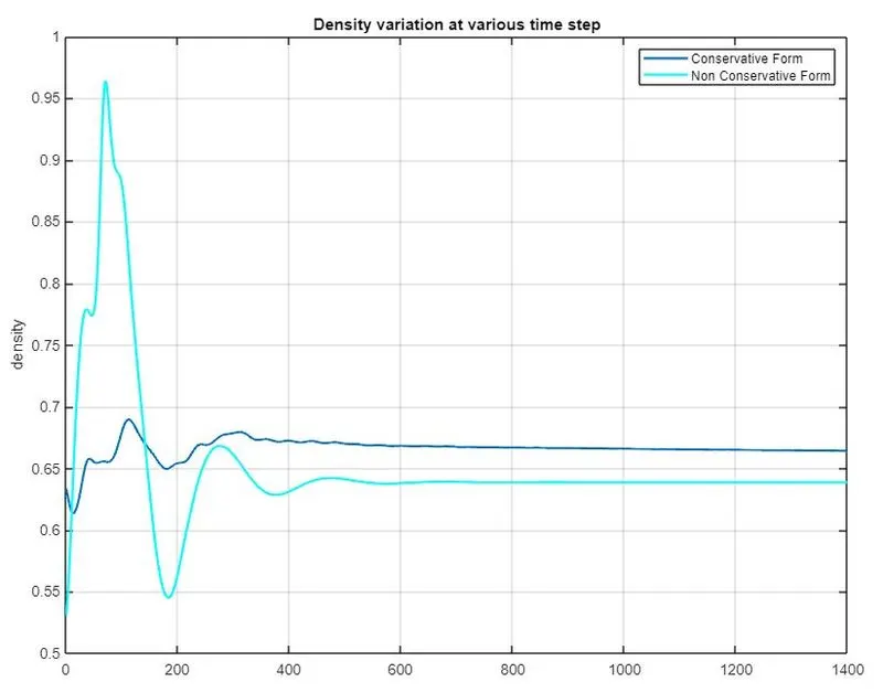
title('Density variation at various time step');
grid on

figure(10)
plot(1:nt,T_throat,'linewidth',0.75);
hold on
plot(1:nt,T_t,'linewidth',0.95)
grid on
ylabel('temeperature');
legend('Conservative Form','Non Conservative Form');
title('Temperature variation at various time step at throat');
grid on


figure(11)

plot(1:nt,pc_throat,'linewidth',0.85)
hold on
plot(1:nt,P_t,'linewidth',0.95)
grid on
ylabel('Presssure');
legend('Conservative Form','Non Conservative Form');
title('Pressure variatiuon at various time step at throat');
grid on

figure(12)
plot(1:nt,Mc_throat,'linewidth',0.85);
hold on
plot(1:nt,M_t,'linewidth',0.90)
grid on
xlabel('Time step');
ylabel('Mach number');
legend('Conservative Form','Non Conservative Form');
title('Mach number variation at various time step at throat');
- Input details are defined such as no of grid points, gamma, CFL, area.
- Independent functions for conservative & non-conservative methods are defined and the results are plotted.
Non Conservative Function Code:
function [V,rho,T,m,M,P,V_t,rho_t,T_t,m_t,M_t,P_t]=non_conservative(throat,x,gamma,dx,A,n,nt,C)

rho =1-0.3146*x;
T=1-0.2314*x;
V=(0.1+1.09*x).*T.^0.5;

dt=min(C.*(dx./(sqrt(T)+V)));

for it=1:nt
    rho_old=rho;
    V_old=V;
    T_old=T;

    for j=2:n-1

        drhodx_p=(rho(j+1)-rho(j))/dx;
        dvdx_p=(V(j+1)-V(j))/dx;
        dtdx_p=(T(j+1)-T(j))/dx;
        dlogA_dx_p=(log(A(j+1))-log(A(j)))/dx;

        %continuity equation
        drhodt_p(j)=-rho(j)*dvdx_p-rho(j)*V(j)*dlogA_dx_p-V(j)*drhodx_p;
        %momentum equation
        dvdt_p(j)=-V(j)*dvdx_p-(1/gamma)*(dtdx_p+(T(j)/rho(j))*drhodx_p);
        %energy equation
        dtdt_p(j)=-V(j)*dtdx_p-(gamma-1)*T(j)*(dvdx_p+V(j)*dlogA_dx_p);
        %solution update
        rho(j)=rho(j)+(drhodt_p(j))*dt;
        V(j)=V(j)+dvdt_p(j)*dt;
        T(j)=T(j)+dtdt_p(j)*dt;
    end

    %corrector step.
    for j=2:n-1
        drhodx_c=(rho(j)-rho(j-1))/dx;
        dvdx_c=(V(j)-V(j-1))/dx;
        dtdx_c=(T(j)-T(j-1))/dx;
        dlogA_dx_c=(log(A(j))-log(A(j-1)))/dx;

        %continuity equation
        drhodt_c(j)=-(rho(j)*dvdx_c)-rho(j)*V(j)*dlogA_dx_c-V(j)*drhodx_c;
        %momentum equation
        dvdt_c(j)=-(V(j)*dvdx_c)-(1/gamma)*(dtdx_c+(T(j)/rho(j))*drhodx_c);
        %energy equation
        dtdt_c(j)=-(V(j)*dtdx_c)-(gamma-1)*T(j)*(dvdx_c+V(j)*dlogA_dx_c);
    end

    %average values
       dvdt=0.5*(dvdt_c+dvdt_p);
       drhodt=0.5*(drhodt_p+drhodt_c);
       dtdt=0.5*(dtdt_c + dtdt_p);

       for i=2:n-1
           rho(i)=rho_old(i)+drhodt(i)*dt;
           V(i)=V_old(i)+dvdt(i)*dt;
           T(i) = T_old(i)+dtdt(i)*dt;
       end
       V(1)=2*V(2)-V(3);
       V(n)=2*V(n-1)-V(n-2);
       rho(n) = 2*rho(n-1)-rho(n-2);
       T(n)=2*T(n-1)-T(n-2);

       m=rho.*A.*V;
       P=rho.*T;
       M=V./sqrt(T);


       rho_t(it)=rho(throat);
       V_t(it)=V(throat);
       T_t(it)=T(throat);
       P_t(it)=P(throat);
       M_t(it)=M(throat);
       m_t(it)=m(throat);

       rho_exact=0.634*ones(1,1400);
       t_exact=0.833*ones(1,1400);
       p_exact = 0.528*ones(1,1400);
       mach_exact=1*ones(1,1400);

       figure(1)
       if it==50
           plot(x,m,'b','linewidth',1.5);
           hold on
        elseif it==100
              plot(x,m,'r','linewidth',1.5);
              hold on
        elseif it==150
               plot(x,m,'c','linewidth',1.5);
               hold on
        elseif  it==300
                plot(x,m,'g','linewidth',1.5);
                hold on
        elseif  it==600
                plot(x,m,'y','linewidth',1.5);
                hold on
        elseif it==900
                plot(x,m,'k','linewidth',1.5);
                hold on
        elseif it==1400
                plot(x,m,'m','linewidth',1.5);
                grid on
       end
end

  xlabel('Non dimensional distance through nozzle (x)','fontsize',10);
  ylabel('Non dimensional mass flow rate through nozzle x','fontsize',10);
  title('Variation of mass flow rate (non conservative form) along x at different steps');
  legend({'50 time steps','100 time steps','150 time steps','300 time steps','600 time steps','900 time steps','1400 time steps'});


end
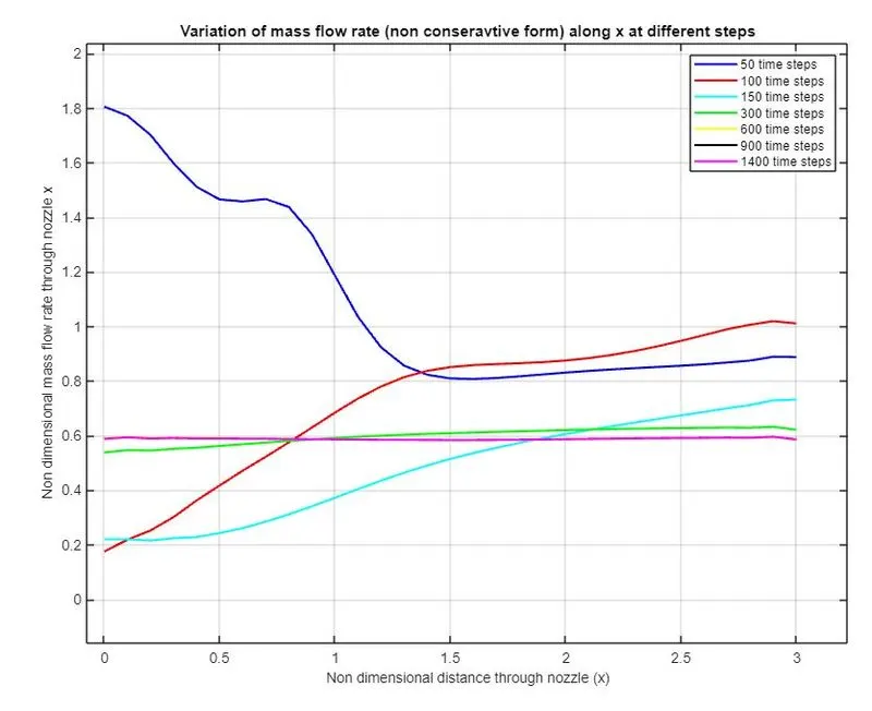
Non Conservative output:
Conservative Function Code:
function [Vc,rhoc,Tc,cons_mass_flow_throat,Mc,pc,Vc_throat,rho_throat,T_throat,cons_mass_flow,Mc_throat,pc_throat]=conservative(throat,x,gamma,dx,A,n,nt,C)
R=8.314;
for i=1:n
    if (x(i)<=0.5)
        rho_in (i)=1;
        T_in(i)=1;
    elseif (x(i)>=0.5) && (x(i) <= 1.5)
            rho_in(i)=1-(0.366*(x(i)-0.5));
            T_in(i)=1-0.167*(x(i)-0.5);
        else
                rho_in(i)=0.634-0.3879*(x(i)-1.5);
                T_in(i)=0.833-0.3507*(x(i)-1.5);
    end
end

 u_in=0.59./(rho_in.*A);
 rhoc = rho_in;
 Tc=T_in;
 Vc=u_in;

dt=0.0206;
t_sim=(nt-1)*dt;
t=0:dt:t_sim;

U1=rhoc.*A;
U2=rhoc.*A.*Vc;
U3=rhoc.*A.*((Tc/(gamma-1))+(0.5*gamma.*Vc.*Vc));

%MacCormack method
for j=1:length(t)
    U1_old=U1;
    U2_old=U2;
    U3_old=U3;

    F1=U2;
    F2=((U2.^2)./U1)+((gamma-1)/gamma).*(U3-((gamma/2)*(U2.^2./U1)));
    F3=((gamma.*U2.*U3)./U1)-((gamma*(gamma-1))/2)*(U2.^3)./(U1.^2);

    %predictor method
    for k=2:n-1
        dA_dx(j)=(A(k+1)-A(k))/dx;
        dlogA_dx = (log(A(k+1))-log(A(k)))/dx;
        J2(k)=dlogA_dx*((gamma-1)/gamma)*(U3(k)-(0.5*gamma*U2(k)^2)/(U1(k)));


        %continuity step

        dF1_dx_p=(F1(k+1)-F1(k))/dx;
        dU1_dt_p(k)=-dF1_dx_p;
        %momentum equation
        dF2_dx_p=(F2(k+1)-F2(k))/dx;
        dU2_dt_p(k)=-dF2_dx_p+J2(k);

        dF3_dx_p=(F3(k+1)-F3(k))/dx;
        dU3_dt_p(k)=-dF3_dx_p;

        U1(k)=(dU1_dt_p(k).*dt)+U1_old(k);
        U2(k)=(dU2_dt_p(k).*dt)+U2_old(k);
        U3(k) = (dU3_dt_p(k).*dt)+U3_old(k);
    end
    %applying boundary condition
    %input
    U1(1)=A(1);
    U2(1)=2*U2(2)-U2(3);
    U3(1)=U1(1)*((Tc(1)/(gamma-1)+((gamma/2)*Vc(1)^2)));
    %output
    U1(n)=2*U1(n-1)-U1(n-2);
    U2(n)=2*U2(n-1)-U2(n-2);
    U3(n)=2*U3(n-1)-U3(n-2);

    rhoc=U1./A;
    Tc=(gamma-1).*((U3./U1)-((gamma/2).*(U2./U1).^2));

    F1=U2;
    F2=((U2.^2)./U1)+((gamma-1)/gamma).*(U3-((gamma/2)*(U2.^2./U1)));
    F3=((gamma.*U2.*U3)./U1)-((gamma*(gamma-1))/2)*(U2.^3)./(U1.^2);

    %corrector method
    for k=2:n-1
        dA_dx(j)=(A(k)-A(k-1))/dx;
        dlogA_dx=(log(A(k))-log(A(k-1)))/dx;
        J2(k)=dlogA_dx*((gamma-1)/gamma)*(U3(k)-(0.5*gamma*U2(k)^2)/(U1(k)));

        %continuity step
        dF1_dx_c=(F1(k)-F1(k-1))/dx;
        dU1_dt_c(k)=-dF1_dx_c;

        %momentum equation
        dF2_dx_c=(F2(k)-F2(k-1))/dx;
        dU2_dt_c(k)=-dF2_dx_c +J2(k);

        %energy equation
        dF3_dx_c=(F3(k)-F3(k-1))/dx;
        dU3_dt_c(k)=-dF3_dx_c;
    end
    for pc=2:n-1
        dU1_dt_avg(pc)=0.5*(dU1_dt_c(pc)+dU1_dt_p(pc));
        dU2_dt_avg(pc)=0.5*(dU2_dt_c(pc)+dU2_dt_p(pc));
        dU3_dt_avg(pc)=0.5*(dU3_dt_c(pc)+dU3_dt_p(pc));

        U1(pc)=(dU1_dt_avg(pc)*dt)+U1_old(pc);
         U2(pc)=(dU2_dt_avg(pc)*dt)+U2_old(pc);
          U3(pc)=(dU3_dt_avg(pc)*dt)+U3_old(pc);
    end

    %boundary

    U1(1)=A(1);
    U2(1)=2*U2(2)-U2(3);
    U3(1)=U1(1)*((Tc(1)/(gamma-1)+((gamma/2)*Vc(1)^2)));
    %input
    U1(n)=2*U1(n-1)-U1(n-2);
    U2(n)=2*U2(n-1)-U2(n-2);
    U3(n)=2*U3(n-1)-U3(n-2);


    rhoc=U1./A;
    Vc=U2./U1;
    Tc=(gamma-1)*((U3./U1)-((gamma/2).*(Vc.^2)));

    pc=rhoc.*Tc;
    Mc=Vc./(Tc.^0.5);
    cons_mass_flow=rhoc.*Vc.*A;
    %variables at throat
    rho_throat(j)=rhoc(throat);
    T_throat(j)=Tc(throat);
    pc_throat(j)=pc(throat);
    Mc_throat(j)=Mc(throat);
    cons_mass_flow_throat(j)=cons_mass_flow(throat);
    Vc_throat(j)=Vc(throat);

    figure(2)
    if j==50
        plot(x,cons_mass_flow,'b','linewidth',1.5);
        hold on
    elseif j==100
        plot(x,cons_mass_flow,'r','linewidth',1.5)
        hold on
    elseif j==150
        plot(x,cons_mass_flow,'c','linewidth',1.5)
        hold on
    elseif j==300
        plot(x,cons_mass_flow,'g','linewidth',1.5)
        hold on
    elseif j==600
        plot(x,cons_mass_flow,'y','linewidth',1.5)
        hold on
    elseif j==900
        plot(x,cons_mass_flow,'*','linewidth',1.5)
        hold on
    elseif j==1400
        plot(x,cons_mass_flow,'m','linewidth',1.5)
        hold on


    end
end
xlabel('Non dimensional distance through nozzle(x)','fontsize',10)
ylabel('Non dimensional mass flow rate through nozzle x','fontsize',10);
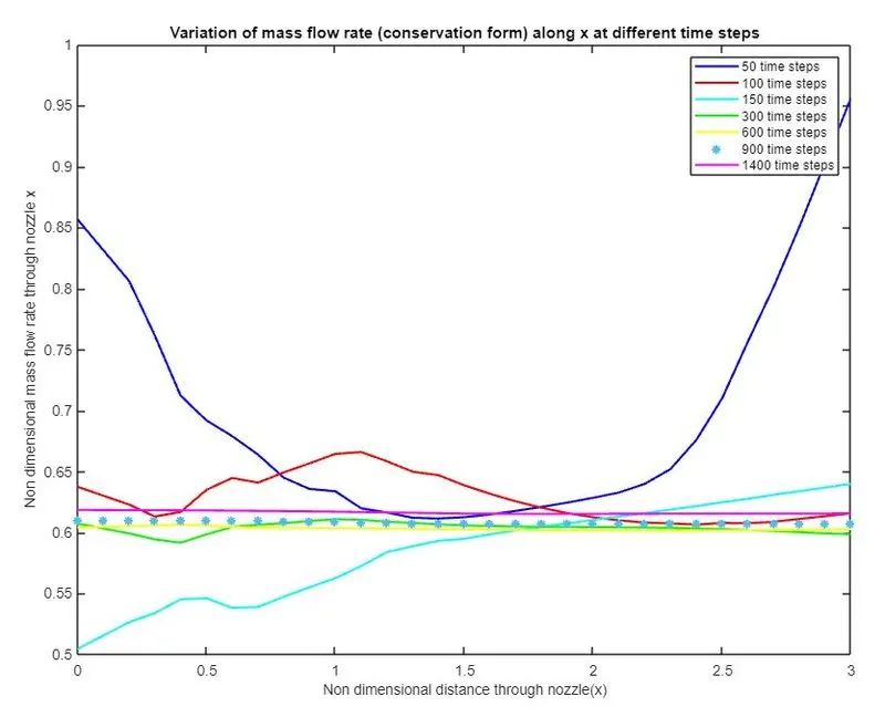
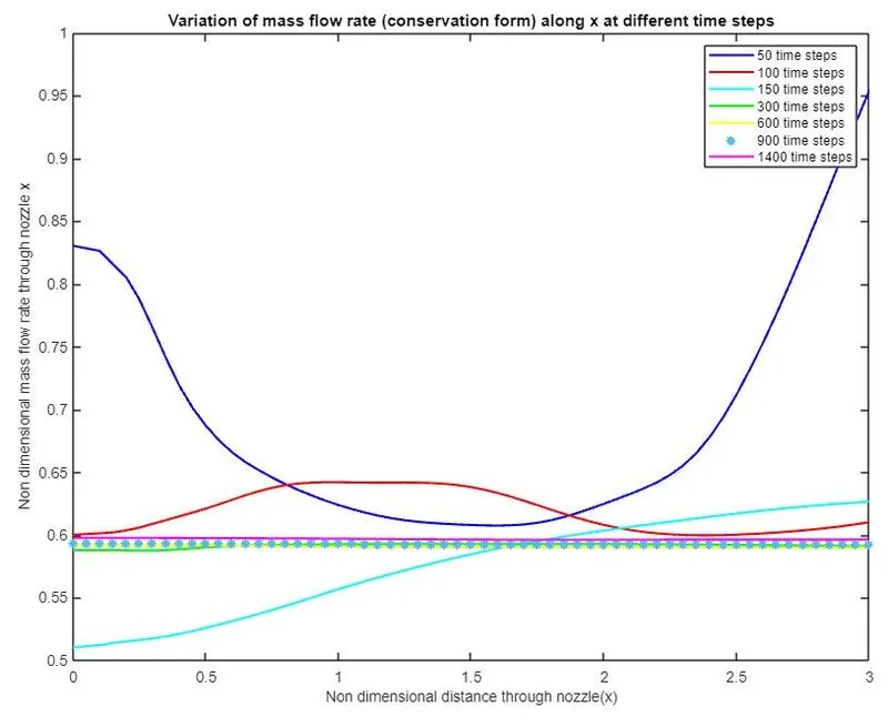
title('Variation of mass flow rate (conservation form) along x at different time steps');
  legend({'50 time steps','100 time steps','150 time steps','300 time steps','600 time steps','900 time steps','1400 time steps'});
end
Conservative function output
Comparison of mass flow rate Plot:
Mach number profile plot:
Pressure profile plot:
Density profile plot:
Temperature profile plot:
Velocity profile plot:
Variation of Density with time step:
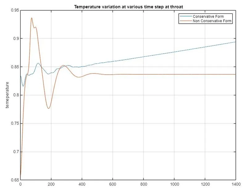
Variation of temperature at throat with time step:
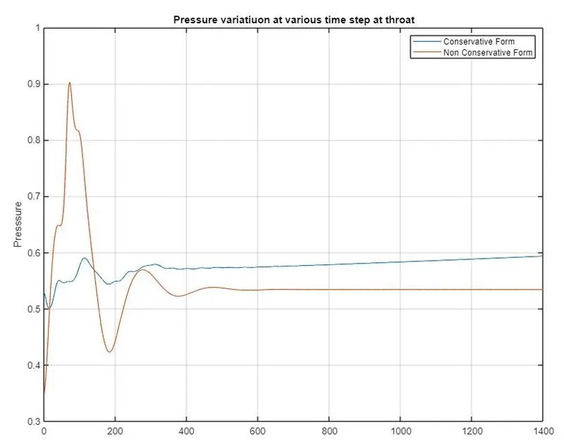
Variation of pressure at throat with time step:
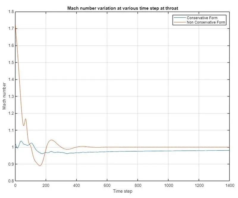
Variation of Mach Number at throat with time step:
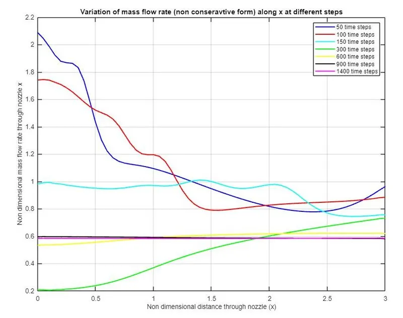
Variation of mass flow rate (Non-conservative form) along X:
Variation of mass flow rate (Conservative form) along X:
Significance of Grid Dependence:
The below table includes the variables at different grid points n=31 & n=61
|
Primitive variables and condition at nozzle |
||||||
|
Density ratio |
Temperature ratio |
Pressure ratio |
Mach number |
|||
|
ρ/ρo |
T/To |
P/Po |
M |
|||
|
n=31 |
non conservative |
0.6387 |
0.8365 |
0.5342 |
0.9994 |
|
|
n=61 |
non conservative |
0.6377 |
0.8354 |
0.5327 |
0.9998 |
|
|
n=31 |
conservative |
0.6642 |
0.8939 |
0.5937 |
0.9801 |
|
|
n=61 |
conservative |
0.6424 |
0.8601 |
0.5525 |
1.0008 |
|
|
Exact solution |
0.634 |
0.833 |
0.528 |
1 |
||
CFL data effect on conservative form for 31 grid points:
|
CFL number |
Density ratio |
Temperature ratio |
Pressure ratio |
Mach number |
|
ρ/ρo |
T/To |
P/Po |
M |
|
|
0.5 |
0.6642 |
0.8939 |
0.5937 |
0.9801 |
|
0.8 |
0.6642 |
0.8939 |
0.5937 |
0.9801 |
|
1 |
0.6642 |
0.8939 |
0.5937 |
0.9801 |
|
1.1 |
0.6642 |
0.8939 |
0.5937 |
0.9801 |
|
1.2 |
0.6642 |
0.8939 |
0.5937 |
0.9801 |
|
Exact solution |
0.634 |
0.833 |
0.528 |
1 |
The CFL value does not have any effecct on primitive variables ration in conservative form
CFL data effect on non conservative form for 31 grid points:
|
CFL number |
Density ratio |
Temperature ratio |
Pressure ratio |
Mach number |
|
ρ/ρo |
T/To |
P/Po |
M |
|
|
0.5 |
0.6387 |
0.8365 |
0.5342 |
0.9994 |
|
0.8 |
0.6393 |
0.8367 |
0.5349 |
0.9991 |
|
1 |
0.6397 |
0.8368 |
0.5353 |
0.9988 |
|
1.1 |
0.6399 |
0.8369 |
0.5355 |
0.9987 |
|
1.2 |
---------- |
----------- |
----------- |
-------- |
|
Exact solution |
0.634 |
0.833 |
0.528 |
1 |
The solution blew at CFL value equal to 1.2
Simulation time data:
|
Grid Points |
Time for Simulation |
|
|
n=31 |
non conservative |
3.151 |
|
n=31 |
conservative |
2.952 |
|
n=61 |
non conservative |
3.2231 |
|
n=61 |
conservative |
3.0038 |
Conclusion:
It is observed that as the number of grid points increases, the resultant value approaches very close to the analytical solution but also increases the simulation time required to run the program.
- The time taken for simulation in case of conservative form is lesser when compared to non conservative form.
- In grid dependence test we observe that the accuracy in case of non conservative form is more as comapared to conservative form as it is very close to exact analytical solution.
- The conservative form provides more accuracy incase of mass flow rate whereas non conservative provide more accuracy in case of primitive variables .
- In general Non conservative form has higher accuracy than conservative form.
- In the non conservative form, it is observed that as CFL value increases the density, pressure and temperature ratio increases, but mach number decreases. And at CFL value 1.2 the sloution blown off.
- In the conservative form, the increase or decrease in CFL value doesnt effect the solution itself.