Week 5.1 - Mid term project - Solving the steady and unsteady 2D heat conduction problem

The 2D steady-state Heat conduction is

(d²T/dx² + d²T/dy²) = 0

((T_L - 2T_P + T_R) / dx²) + ((T_T - 2T_P + T_B) / dy²) = 0

2T_P / dx² + 2T_P/dy² = ((T_L + T_R) / dx²) + (( T_T +T_B) / dy²)

Tp = (1/K)*[((T_R + T_L)/dx²) + ((T_T + T_B)/dy²)

K = 2((dx²+dy²)/(dx²*dy²))

Transient Form:

dT/dt + α*∇(T) = 0

((T_i,jⁿ⁺¹ - T_i,jⁿ)/dt) + α (d²T/dx² + d²T/dy²) = 0

((T_i,jⁿ⁺¹ - T_i,jⁿ)/dt) + α((T_i+1,j - 2T_i,j + T_i-1,j)/dx² + (T_i,j+1 - 2T_i,j + T_i,j-1)/dy² ) = 0

T_Pⁿ⁺¹ = T_Pⁿ + α*dt ((T_R - 2T_P + T_L) / dx²) + ((T_T - 2T_P + T_B) / dy²)

T_Pⁿ⁺¹ = T_Pⁿ + K1 (T_Rⁿ - 2T_Pⁿ + T_Lⁿ) + K2 ( T_Tⁿ - 2T_Pⁿ + T_Bⁿ) ; K1 = α*dt/dx² ; K2 = α*dt/dy²;

The above equation is evaluated @ time step n, hence explicit form

Implicit form of the same equation is as shown below:

T_Pⁿ⁺¹ = T_Pⁿ + K1 (T_Rⁿ⁺¹ - 2T_Pⁿ⁺¹ + T_Lⁿ⁺¹) + K2 ( T_Tⁿ⁺¹ - 2T_Pⁿ⁺¹ + T_Bⁿ⁺¹) ; K1 = α*dt/dx² ; K2 = α*dt/dy²;

Matlab Code:

Top boundary temperature 600 K

Bottom Boundary temperature 900 K

Left Boundary temperature 400 K

Right Boundary temperature 800 K

error 1e-4

Steady state heat conduction

- Inputs & constanst are defined into variables.

- Boundary conditions are defined

- Code is equipped with if-else loop, while loop & for loops.

- Temperature distribution graph is obtained through conturf command.

clear all
close all 
clc

% Domain length & no of node
n = 10;
l = 1;
x = linspace(0,l,n);
y = linspace(0,l,n);
dx = l/(n-1);
dy = l/(n-1);


% Defining temp array
T = 400*ones(n,n);

% Initial BC at left and right
T(1:end,1) = 400;
T(1:end,end) = 800;

% Initial BC at bottom and top
T(end,1:end) = 900;
T(1,1:end) = 600;

% Initial conditions at corners by averaging neighbouring values
T(1,1) = 500;
T(end,1) = 650;
T(1,end) = 700;
T(end,end) = 850;

T_old = T;

% Defining constant
K = (2*(dx^2+dy^2))/(dx^2*dy^2);
alpha = 1.2;

error = 10;
tol = 1e-4; % absolute err criteria as defined
iter_count = 0;

% input command to get user input

method = input('Enter(1) for jacobi,(2) for gauss siediel,(3) for sos');
if method == 1
    while(error>tol)
        for i = 2:n-1
            for j = 2:n-1
            term1 = (T_old(i+1,j)+T_old(i-1,j))/dx^2;
            term2 = (T_old(i,j+1)+T_old(i,j-1))/dy^2;
            T(i,j) = (term1+term2)/K;
            end
        end
        error = max(max(abs(T_old-T)));
        T_old = T;
        iter_count = iter_count+1;
        
    end
elseif method == 2
    while(error>tol)
        for i = 2:n-1
            for j = 2:n-1
            term1 = (T_old(i+1,j)+T(i-1,j))/dx^2;
            term2 = (T_old(i,j+1)+T(i,j-1))/dy^2;
            T(i,j) = (term1+term2)/K;
            end
        end
        error = max(max(abs(T_old-T)));
        T_old = T;
        iter_count = iter_count+1;
    end
    
else % if method == 3 for SOR
    while(error>tol)
        for i = 2:n-1
            for j = 2:n-1
            term1 = (T_old(i+1,j)+T(i-1,j))/dx^2;
            term2 = (T_old(i,j+1)+T(i,j-1))/dy^2;
            T(i,j) = ((1-alpha)*T_old(i,j))+(alpha*((term1+term2)/K));
            end
        end
        error = max(max(abs(T_old-T)));
        T_old = T;
        iter_count = iter_count+1;
        
    end
end

% Plotting the result 

[X,Y] = meshgrid(x,y); % to create 2D grid points
contourf(X,Y,T)
colorbar
set(gca,'ydir','reverse') % reversing y axis direction

if method == 1
    title("Jacobi Iteration")
else if method == 2
    title("Gauss Siediel Iteration")
else 
    title("SOR Iteration")
end
end

Transient heat conduction

- Inputs & constanst are defined into variables.

- Boundary conditions are defined

- Code is equipped with if-else loop, while loop & for loops.

- Temperature distribution graph is obtained through conturf command.

clear all
close all 
clc

% Domain length & nodes
n = 10;
l = 1;
x = linspace(0,l,n);
y = linspace(0,l,n);
dx = (l/n-1);
dy = (l/n-1);
dt = 1/10;


T = 400*ones(n,n);

% Initia boundary conditions at left and right
T(1:end,1) = 400;
T(1:end,end) = 800;

% Initia boundary conditions at bottom and top
T(end,1:end) = 900;
T(1,1:end) = 600;

%average values of T at corner boundaries
T(1,1) = 500;
T(end,1) = 650;
T(1,end) = 700;
T(end,end) = 850;


T_old = T;
T_prev = T;

%constants 
alpha = 1.5;
omegha = 1.15;
K1 = (alpha*dt)/(dx^2);
K2 = (alpha*dt)/(dy^2);
iteration = 0;


approach = input('Enter 1 for implicit or Enter 2 for explicit')

if approach == 1
    method = input('Enter 1 for jacobi or 2 for gauss siedel or 3 for sos')
    if method == 1
        for nt = 1:1500
            error = 10;
            tol = 1e-4;
            while(error>tol)
                for i = 2:n-1
                    for j = 2:n-1
                        term1 = 1/(1+(2*K1)+(2*K2));
                        term2 = K1*(T_old(i+1,j)+T_old(i-1,j));
                        term3 = K2 *(T_old(i,j+1)+T_old(i,j-1));
                        T(i,j) = term1*(T_prev(i,j)+term2+term3);
                    end
                end
                iteration = iteration+1;
                error = max(max((abs(T_old-T))));
                T_old = T;
            end
            T_prev = T;
        end
    elseif method ==2
        for nt = 1:1500
            error = 10;
            tol = 1e-4;
            while(error>tol)
                for i = 2:n-1
                    for j = 2:n-1
                        term1 = 1/(1+(2*K1)+(2*K2));
                        term2 = K1*(T_old(i+1,j)+T(i-1,j));
                        term3 = K2 *(T_old(i,j+1)+T(i,j-1));
                        T(i,j) = term1*(T_prev(i,j)+term2+term3);
                    end
                end
                iteration = iteration+1;
                error = max(max(abs(T_old-T)));
                T_old = T;
                
            end
            T_prev = T;
        end
    else
        for nt = 1:1500
            error = 10;
            tol = 1e-4;
            while(error>tol)
                for i = 2:n-1
                    for j = 2:n-1
                        term1 = 1/(1+(2*K1)+(2*K2));
                        term2 = K1*(T_old(i+1,j)+T(i-1,j));
                        term3 = K2 *(T_old(i,j+1)+T(i,j-1));
                        term4 = term1*(T_prev(i,j)+term2+term3);
                        T(i,j)=(1-omegha)*T_old(i,j)+(omegha*term4);
                    end
                end
                iteration = iteration+1;
                error = max(max(abs(T_old-T)));
                T_old = T;
            end
            T_prev = T;
        end
    end
else
     for nt = 1:1500
        for i = 2:n-1
            for j = 2:n-1
                term1 = K1*(T_prev(i+1,j)-2*T_prev(i,j)+T_prev(i-1,j));
                term2 = K2*(T_prev(i,j+1)-2*T_prev(i,j)+T_prev(i,j-1));
                T(i,j) = T_prev(i,j)+term1+term2;
            end
        end
        T_prev = T;
        iteration = iteration+1;
    end
end

% Plotting the result 

[X,Y] = meshgrid(x,y);
figure(1)
contourf(X,Y,T)
colorbar
set(gca,'ydir','reverse')

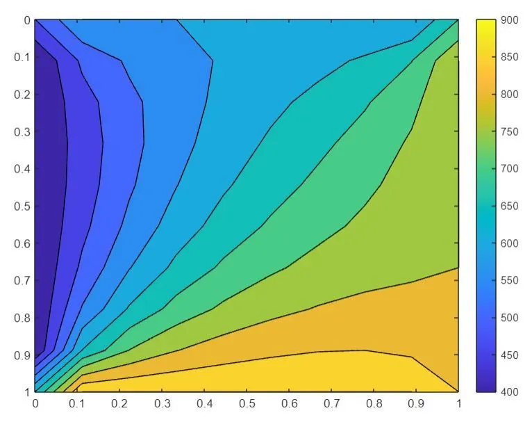
Graph Result:

- The top, bottom, left, and right side of the graphs representing their respective boundary conditions.

- The temperature distribution plot obtained for both the steady and unsteady conditions is the same.

Because in Transient analysis also, the solution approaches to steady-state.

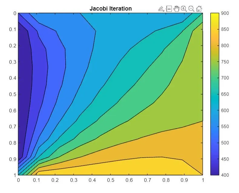
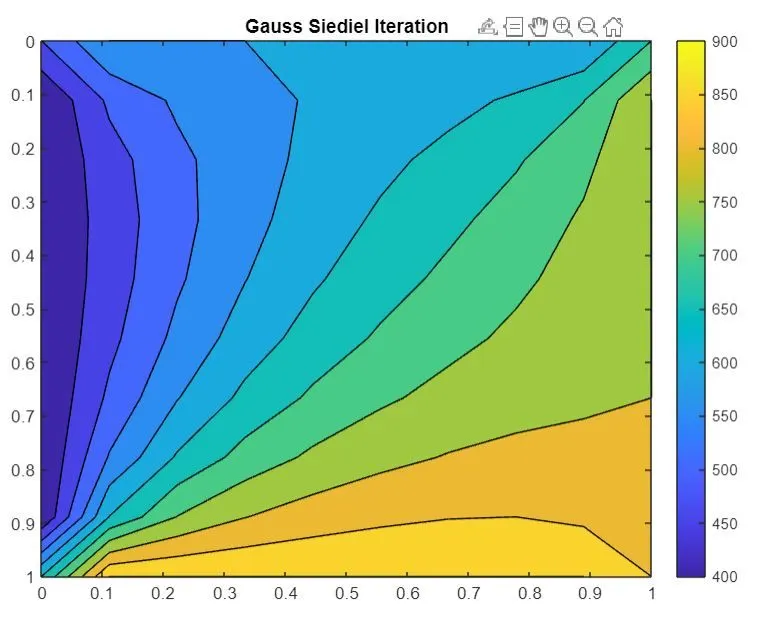
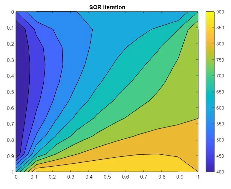
Transient state (Implicit & Explicit)

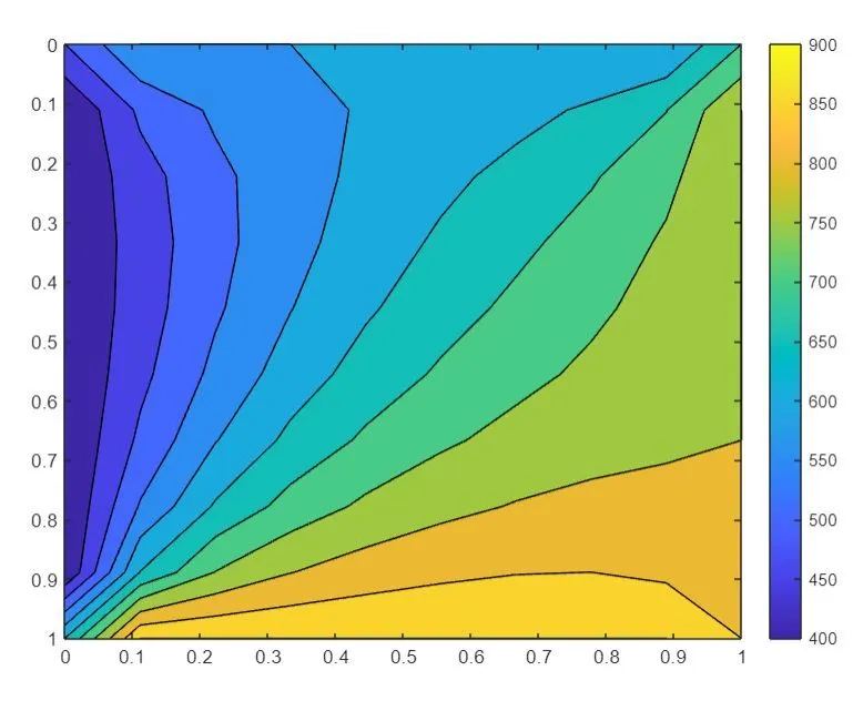
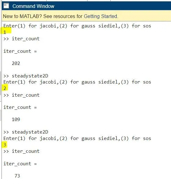
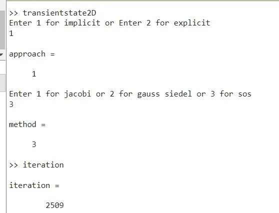
Comparison of number of iterations taken to converge to the solution

Steady state:

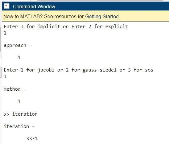
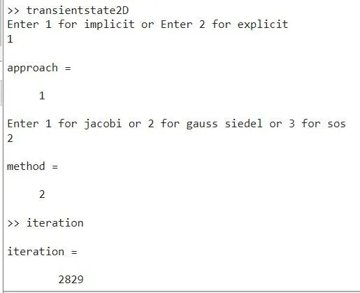
Transient State:

Implicit approach

Explicit approach

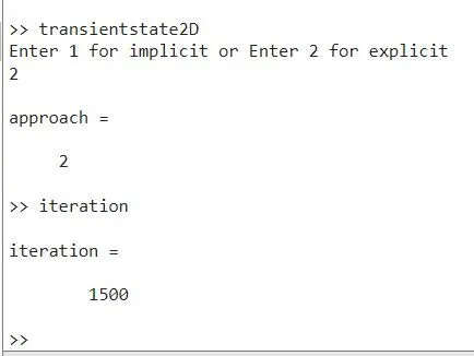
- Number of iteration by the Successive over-relaxation method is less in both steady and transient analysis.

- Successive over relaxaton < Gauss-siedel < Jacobi

- As the explicit approach calculates the solution at a given time step based on the values of the previous time step, the no of iterations is noted less.

- The more complex a calculation is, the more iterations it will take to converge.