Week 7 - Simulation of a 1D Supersonic nozzle flow simulation using Macormack Method
AIM:
To write a Matlab program to simulate the isentropic flow through a quasi 1D subsonic-supersonic nozzle by both the conservation and non-conservation forms of the governing equations and to solve them using the MacCormack's technique.
OBJECTIVE:
- To write a Matlab program to simulate the isentropic flow through a quasi 1D subsonic-supersonic nozzle.
- To solve the problem by MacCormack's technique considering both the conservation and non-conservation forms of the governing equations.
- To plot steady state distribution and time wise variation of primitive variables inside the nozzle.
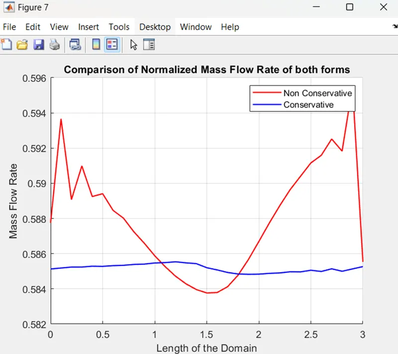
- To compare the mass flow rate at steady state for both conservation form and non-conservation form.
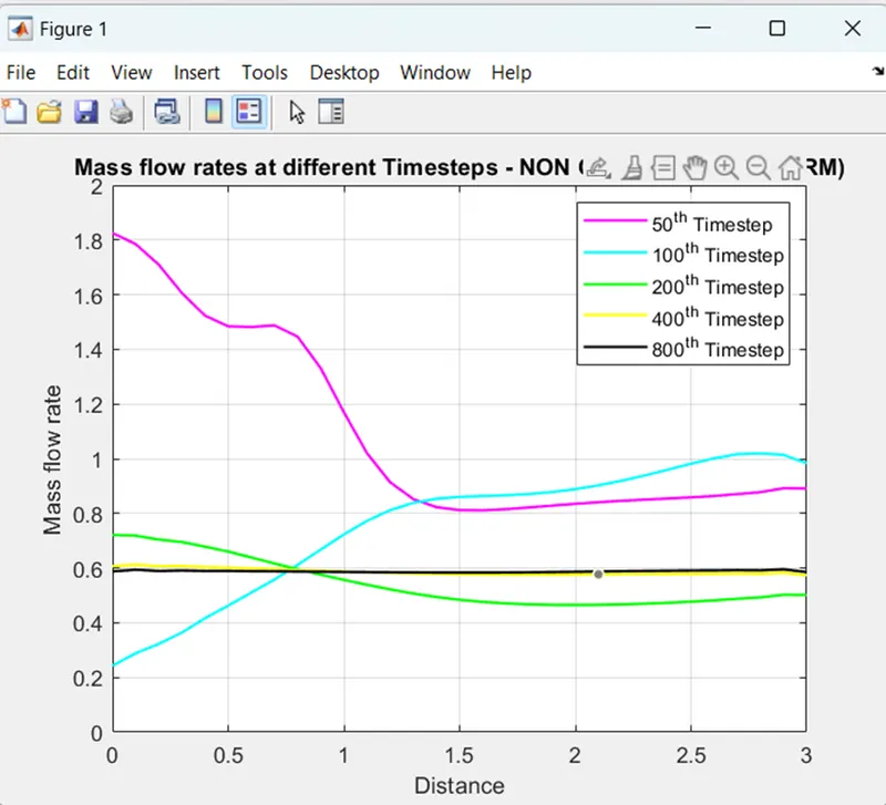
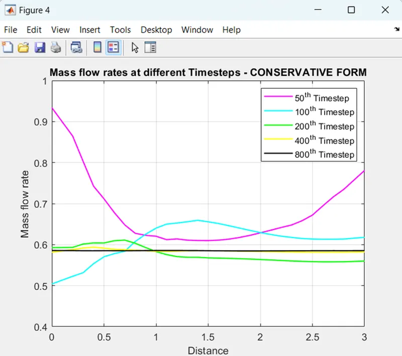
- To plot the variation of Mass flow rate distribution inside the nozzle at different time steps during the time-marching process.
- To perform a grid independence test on the solution.
Theory:
Nozzle:
Step-1 - Governing equations
for Non conservetive :
CONTINUTY EQUATION
dp/dt'=p'dv'/dx'-pv' d(lnA')/dx'-v'dp'/dx'
MOMENTUM ERQUATION
dv'/dt'=-v'dv'/dx'-1/y(dt'/dx'+t'/p' dp'/dx')
ENERGY EQUATION
dT'/dt'=-v'dt'/dx'-(y-1)t'[dv'/dx'+v'd(lnA')/dx'
for conservative equation
CONTINUTY EQUATION
d(p'A')/dt'+d(P'A'V')/dt'=0
MOMENTUM EQUATION
d(p'A'V')/dt'+d[p'A'V'2+(1/Y)P'A'/dx'=1/y p'dA'/dx'
ENERGY EQUATION
d[(e'/y-1+y/2 v'2)A']/dt'+d[p'(e'/y-1+y/2v'2)v'A'+p'A'V']/dx'=0
PREDICTOR STEP
(df/dt)p=f(i+1)-f(i)/dx
SOLUTION STEP
fp=f initial+(df/dt)p.dx
CPRRECTOR STEP
(dfp/dt)c=f(i)-f(i-1)/dx
AVERAGE DERIVATIVE
(dfp/dt)avg=((df/dt)p+(dfp/dt)c)
FINAL SOLUTION UPDATE
fsol=finitial+(df/dt)avg.dt
INITIAL CONDITION
{P=1,T=1}FOR 0
p=1-0.366(x-0.5) for 0.5
t=1-0.167(x-0.5)
p=0.634-0.3879(x-1.5) for 1.5<3.5
v=o.59/pA
nozzle sgape A1+2.2(X-1.5
BOUNDARY CONDITION
INLET
U2(i=1)2u2(i=2)-u2(i=3)
u3is also updated by using the value of updated V
OUTLET
all the three varaible are float
(U1)=2(U1)N-1(U1)N-2
(U2)N=2(U2)N-1-(U2)N-2
(U3)N=2(U3)N-1-(U3)N-3
Explanation:
• To enable a fresh run without changing the previously used values, the code is executed using the clear all, close all, and clc commands.
The input parameters for the variables x, dx, n, gamma, nt, and C are given.
• Using the essential inputs, which are listed below in this section, the non-conservative and conservative forms are created as distinct functions.
• To determine the amount of time that has passed between functions, use the tic toc command.
For the ensuing resolution, rendering is completed
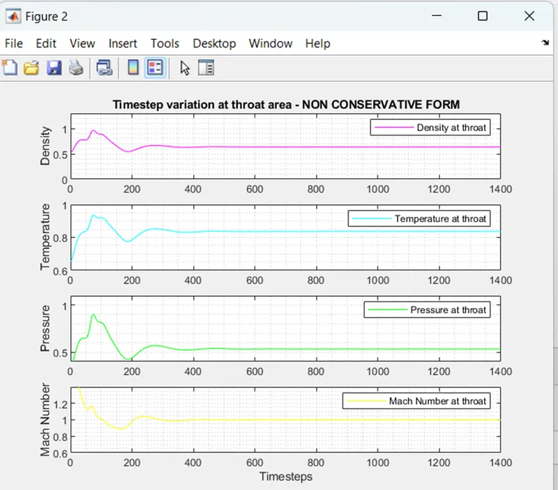
1) Changes in the time step in both types' throat regions
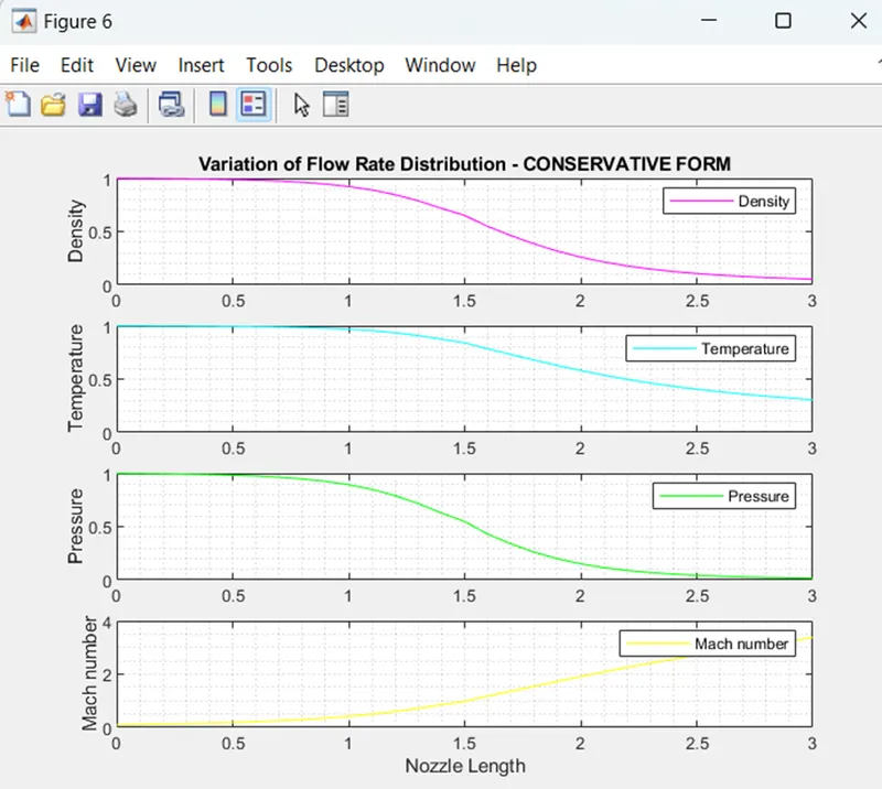
2) Changes in both kinds' flow distribution
3) Evaluation of both types' normalised mass flow rates
Each graphic is computed using four simple variables, such as density, temperature, pressure, and throat Mach number, as well as convergent/divergent sections.
NON COSERVETIVE FORM
Non-Conservative Form
Mass flow rates at different Timesteps:
Non Conservative form:
Explanation:
• The for loop assigns the predictor and corrector techniques separately to compute the values.
Conservative Form
Conservative Form
Observation:
by observing the above plots wecan see that both the forms are in same phase giving the exact same solution for all the values.
Mass flow rates at different Timesteps:
Non Conservative form:
Conservative form:
Observation:
Above plots shows that Mass Flow Rate at different Time steps along the Distance oscillates initially, however the solution becomes stable after the 400th Timestep for both the forms attaining a constant value.
GRID DEPENDENCE TEST:
GRID DEPENDENCE TEST(comparision of solution after 1400 steps)
TYPES OF GRID POINT DENSITY PRESSURE TEMPRATURE MACH TIME ELAPSEDObservation:
• Grid reliance has a significant role in deciding how quickly a problem may be handled. Therefore, we filled the page with 61 grid points instead of the previous 31.
It is evident from the table above that even if the grid points (n) change from 31 to 61, the values are nearly same for all basic variables for both forms, demonstrating that the increase in grid points is unaffected.
• Therefore, it is acceptable to say that the aforementioned issue is grid-dependent.
CONCLUSION:
When all of the aforementioned findings are put together, it is clear that the conservative form converges a little bit quicker than the non-conservative form, which provides a stable solution throughout the simulation. However, both methods are trustworthy for calculating a result that is almost accurate.