Week 7 - Simulation of a 1D Supersonic nozzle flow simulation using Macormack Method
Governing equations:
Non conservative form
Continuity equation
`(delrho)/(delt) = -rho*(delV)/(delx)-rho*V*(del(lnA))/(delx)-V(delrho)/(delx)`
Momentum equation
`(delV)/(delt) = -V*(delV)/(delx)-(1/gamma)*[(delT)/(delx)+(T/rho)*(delrho)/(delx)]`
Energy equation
`(delT)/(delt) = -V*(delT)/(delx)-(gamma-1)*T*[(delV)/(delx)+V(del(lnA))/(delx)]`
Conservative form
Continuity equation
`(del(rho*A))/(delt)-(del(rho*A*V))/(delx)=0`
Momentum equation
`(del(rho*A*V))/(delt) + (del(rho*A*V^2+(1/gamma)*p*A))/(delx)=(1/gamma)*p*(delA)/(delx)`
Energy equation
`(del[rho*(e/(gamma-1)+gamma/2*V^2)*A])/(delt)+(del[rho*(e/(gamma-1)+gamma/2*V^2)*A*V+p*A*V])/(delx)=0`
`U1 = rho'*A'`
`U2=rho'*A'*V'`
`U3=rho'*((e')/(gamma-1)+gamma/2*V'^2)A'`
`F1=rho'*A'*V'`
`F2=rho'*A'*V'^2+1/gamma*p'*A'`
`F3=rho'*((e')/(gamma-1)+gamma/2*V'^2)V'*A' + p'*A'*V'`
`J2=1/gamma*p'*(delA')/(delx')`
From the above equoations we can write that
`(delU1)/(delt')=-(delF1)/(delx')`
`(delU2)/(delt')=-(delF2)/(delx')+J2`
`(delU3)/(delt')=-(delF3)/(delx')`
Above equations we wish to solve numerically by using the MacCormacks technique.
Initial conditions at t=0
`A = 1 + 2.2*(x-1.5)^2` 0<=x<=3
`rho = 1-0.3146*x`
`T = 1-0.2314*x`
`V= (0.1+1.09*x)*T^0.5`
`P = rho*T`
Mach number `M = mu/T^0.5`
Next we come to predictor step:
This is a kind of descritisation step.Where we descretize with forward difference equation.
Next step is the corrector method:
Here we use the backward differencing scheme and rest remains same as that of the predictor method.
Calculation of Average:
Its basically the half of the sum of corrector and predictor value.
Then finally the corrected values at time is t+ Δt
MAIN PROGRAM
close all
clear all
clc

%input parameters
n=31;
x=linspace(0,3,n);
dx=x(2)-x(1);
gamma=1.4;
CFL=0.5;
Area=1+2.2*(x-1.5).^2;
throat=((n+1)/2);
nt=1400;

%main body
tic;
[V,rho,T,m,M,P,V_t,rho_t,T_t,m_t,M_t,P_t]=non_conservative(throat,x,gamma,dx,Area,n,nt,CFL);
non_conservative=toc;

tic
[Vc,rhoc,Tc,cons_mass_flow_throat,Mc,pc,Vc_throat,rho_throat,T_throat,cons_mass_flow,Mc_throat,pc_throat]=conservative(throat,x,gamma,dx,Area,n,nt,CFL);
conservative=toc;

%plotting
figure(3)
plot(x,m,'linewidth',1);
hold on;
plot(x,cons_mass_flow,'--');
%exact analytical solution rho*A*v=0.579
plot(x,linspace(0.579,0.579,n),'*','linewidth',1);
xlabel('Distance of nozzle (x)');
ylabel('Mass flow rate');
legend('Non conservative form','Conservative form','Exact analytical solution');
title('Comparision of mass flow rate(conventional form vs non conventional');
grid on ;

figure(4)
plot(x,M,'linewidth',1);
hold on
plot(x,Mc,'--','linewidth',1,'color','g');
grid on
xlabel('Distance of nozzle(x)');
ylabel('Mach number');
legend('Non conservative form','Conservative form');
title('Mach number profile');
grid on

figure(5)
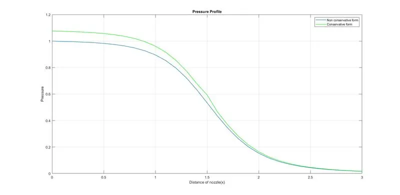
plot(x,P,'linewidth',1);
hold on
plot(x,pc,'g','linewidth',1);
grid on
xlabel('Distance of nozzle(x)');
ylabel('Pressure');
legend('Non conservative form','Conservative form');
title('Pressure Profile');
grid on

figure(6)
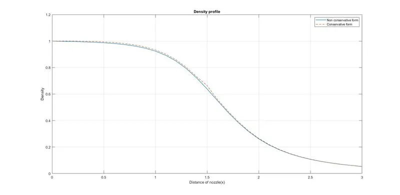
plot(x,rho,'linewidth',1)
hold on
plot(x,rhoc,'--','linewidth',1);
grid on
xlabel('Distance of nozzle(x)');
ylabel('Density');
legend('Non conservative form','Conservative form');
title('Density profile');
grid on

figure(7)
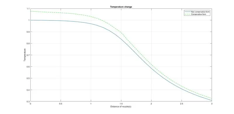
plot(x,T,'linewidth',1);
hold on
plot(x,Tc,'--','linewidth',1,'color','g');
grid on
xlabel('Distance of nozzle(x) ');
ylabel('Temperature');
legend('Non conservative form','Conservative form');
title('Temperature change');

figure(8)
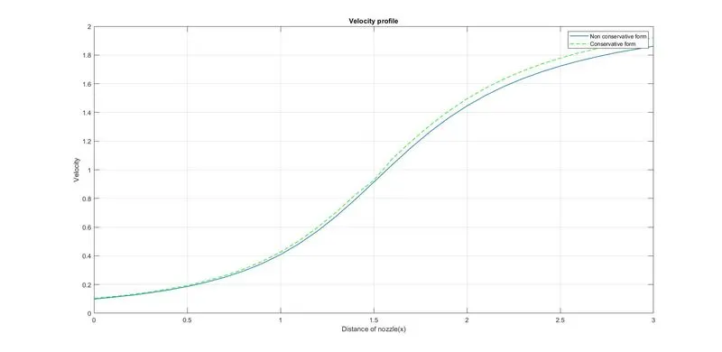
plot(x,V,'linewidth',1.0);
hold on ;
plot(x,Vc,'--','linewidth',1,'color','g');
grid on
xlabel('Distance of nozzle(x)');
ylabel('Velocity');
legend('Non conservative form','Conservative form');
title('Velocity profile');
grid on

figure(9)
plot(1:nt,rho_throat,'linewidth',1);
hold on
plot(1:nt,rho_t,'c','linewidth',1);
grid on
ylabel('Density');
legend('Conservative form','Non conservative form');
title('Density variation at various time step');
grid on

figure(10)
plot(1:nt,T_throat,'linewidth',1);
hold on
plot(1:nt,T_t,'linewidth',1)
grid on
ylabel('Temeperature');
legend('Conservative form','non Conservative form');
title('Temperature variation at various time step at throat');
grid on

figure(11)
plot(1:nt,pc_throat,'linewidth',1)
hold on
plot(1:nt,P_t,'linewidth',1)
grid on
ylabel('Presssure');
legend('Conservative form','Non conservative form');
title('Pressure variatiuon at various time step at throat');
grid on

figure(12)
plot(1:nt,Mc_throat,'linewidth',1);
hold on
plot(1:nt,M_t,'linewidth',1)
grid on
xlabel('Time step');
ylabel('Mach number');
legend('Conservative form','Non conservative form');
title('Mach number variation at various time step at throat');- The input parameters were defined like the number of grid points, gamma, CFL and area function etc.
- The non conservative function were called to obtain all the data about the variables .
- The conservative function were called to obtain all the data about the variables .
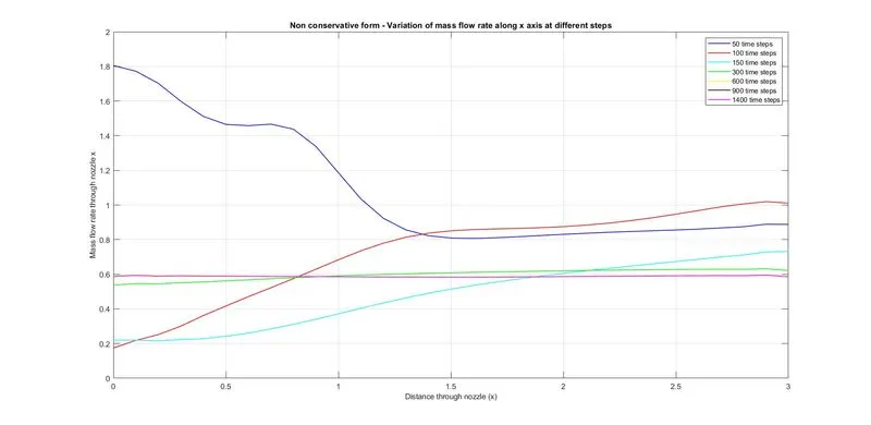
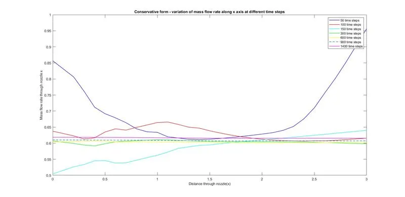
- To visualise the result both the conservative and non conservative data were erpresented in graph form.
FUNCTION CODES:
CONSERVATIVE
%conservative form
function [Vc,rhoc,Tc,cons_mass_flow_throat,Mc,pc,Vc_throat,rho_throat,T_throat,cons_mass_flow,Mc_throat,pc_throat]=conservative(throat,x,gamma,dx,A,n,nt,C)

R=8.314;
for i=1:n
    if (x(i)<=0.5)
        rho_in (i)=1;
        T_in(i)=1;
    elseif (x(i)>=0.5) && (x(i) <= 1.5)
            rho_in(i)=1-(0.366*(x(i)-0.5));
            T_in(i)=1-0.167*(x(i)-0.5);
        else
                rho_in(i)=0.634-0.3879*(x(i)-1.5);
                T_in(i)=0.833-0.3507*(x(i)-1.5);
    end
end

 u_in=0.59./(rho_in.*A);
 rhoc = rho_in;
 Tc=T_in;
 Vc=u_in;

dt=0.0206;
t_sim=(nt-1)*dt;
t=0:dt:t_sim;

U1=rhoc.*A;
U2=rhoc.*A.*Vc;
U3=rhoc.*A.*((Tc/(gamma-1))+(0.5*gamma.*Vc.*Vc));

%Macormack method
for j=1:length(t)
    U1_old=U1;
    U2_old=U2;
    U3_old=U3;

    F1=U2;
    F2=((U2.^2)./U1)+((gamma-1)/gamma).*(U3-((gamma/2)*(U2.^2./U1)));
    F3=((gamma.*U2.*U3)./U1)-((gamma*(gamma-1))/2)*(U2.^3)./(U1.^2);

    %predictor method
    for k=2:n-1
        dA_dx(j)=(A(k+1)-A(k))/dx;
        dlogA_dx = (log(A(k+1))-log(A(k)))/dx;
        J2(k)=dlogA_dx*((gamma-1)/gamma)*(U3(k)-(0.5*gamma*U2(k)^2)/(U1(k)));

        %continuity step

        dF1_dx_p=(F1(k+1)-F1(k))/dx;
        dU1_dt_p(k)=-dF1_dx_p;
        %momentum equation
        dF2_dx_p=(F2(k+1)-F2(k))/dx;
        dU2_dt_p(k)=-dF2_dx_p+J2(k);

        dF3_dx_p=(F3(k+1)-F3(k))/dx;
        dU3_dt_p(k)=-dF3_dx_p;

        U1(k)=(dU1_dt_p(k).*dt)+U1_old(k);
        U2(k)=(dU2_dt_p(k).*dt)+U2_old(k);
        U3(k) = (dU3_dt_p(k).*dt)+U3_old(k);
    end
    %applying boundry condition
    %input
    U1(1)=A(1);
    U2(1)=2*U2(2)-U2(3);
    U3(1)=U1(1)*((Tc(1)/(gamma-1)+((gamma/2)*Vc(1)^2)));
    %output
    U1(n)=2*U1(n-1)-U1(n-2);
    U2(n)=2*U2(n-1)-U2(n-2);
    U3(n)=2*U3(n-1)-U3(n-2);

    rhoc=U1./A;
    Tc=(gamma-1).*((U3./U1)-((gamma/2).*(U2./U1).^2));

    F1=U2;
    F2=((U2.^2)./U1)+((gamma-1)/gamma).*(U3-((gamma/2)*(U2.^2./U1)));
    F3=((gamma.*U2.*U3)./U1)-((gamma*(gamma-1))/2)*(U2.^3)./(U1.^2);

    %corrector method
    for k=2:n-1
        dA_dx(j)=(A(k)-A(k-1))/dx;
        dlogA_dx=(log(A(k))-log(A(k-1)))/dx;
        J2(k)=dlogA_dx*((gamma-1)/gamma)*(U3(k)-(0.5*gamma*U2(k)^2)/(U1(k)));

        %continuity step
        dF1_dx_c=(F1(k)-F1(k-1))/dx;
        dU1_dt_c(k)=-dF1_dx_c;

        %momentum equation
        dF2_dx_c=(F2(k)-F2(k-1))/dx;
        dU2_dt_c(k)=-dF2_dx_c +J2(k);

        %energy equation
        dF3_dx_c=(F3(k)-F3(k-1))/dx;
        dU3_dt_c(k)=-dF3_dx_c;
    end
    for pc=2:n-1
        dU1_dt_avg(pc)=0.5*(dU1_dt_c(pc)+dU1_dt_p(pc));
        dU2_dt_avg(pc)=0.5*(dU2_dt_c(pc)+dU2_dt_p(pc));
        dU3_dt_avg(pc)=0.5*(dU3_dt_c(pc)+dU3_dt_p(pc));

        U1(pc)=(dU1_dt_avg(pc)*dt)+U1_old(pc);
         U2(pc)=(dU2_dt_avg(pc)*dt)+U2_old(pc);
          U3(pc)=(dU3_dt_avg(pc)*dt)+U3_old(pc);
    end

    %boundry
    %input
    U1(1)=A(1);
    U2(1)=2*U2(2)-U2(3);
    U3(1)=U1(1)*((Tc(1)/(gamma-1)+((gamma/2)*Vc(1)^2)));
    %input
    U1(n)=2*U1(n-1)-U1(n-2);
    U2(n)=2*U2(n-1)-U2(n-2);
    U3(n)=2*U3(n-1)-U3(n-2);

    rhoc=U1./A;
    Vc=U2./U1;
    Tc=(gamma-1)*((U3./U1)-((gamma/2).*(Vc.^2)));

    pc=rhoc.*Tc;
    Mc=Vc./(Tc.^0.5);
    cons_mass_flow=rhoc.*Vc.*A;

    %variables at throat
    rho_throat(j)=rhoc(throat);
    T_throat(j)=Tc(throat);
    pc_throat(j)=pc(throat);
    Mc_throat(j)=Mc(throat);
    cons_mass_flow_throat(j)=cons_mass_flow(throat);
    Vc_throat(j)=Vc(throat);

    figure(2)
    if j==50
        plot(x,cons_mass_flow,'b','linewidth',1);
        hold on
    elseif j==100
        plot(x,cons_mass_flow,'r','linewidth',1)
        hold on
    elseif j==150
        plot(x,cons_mass_flow,'c','linewidth',1)
        hold on
    elseif j==300
        plot(x,cons_mass_flow,'g','linewidth',1)
        hold on
    elseif j==600
        plot(x,cons_mass_flow,'y','linewidth',1)
        hold on
    elseif j==900
        plot(x,cons_mass_flow,'--','linewidth',1)
        hold on
    elseif j==1400
        plot(x,cons_mass_flow,'m','linewidth',1)
        hold on


    end
end
xlabel('Distance through nozzle(x)','fontsize',10)
ylabel('Mass flow rate through nozzle x','fontsize',10);
title('Conservative form - variation of mass flow rate along x axis at different time steps');
  legend({'50 time steps','100 time steps','150 time steps','300 time steps','600 time steps','900 time steps','1400 time steps'});
end
NON CONSERVATIVE
%function for non-conservative form

function [V,rho,T,m,M,P,V_t,rho_t,T_t,m_t,M_t,P_t]=non_conservative(throat,x,gamma,dx,A,n,nt,C)

%calculation

rho =1-0.3146*x;
T=1-0.2314*x;
V=(0.1+1.09*x).*T.^0.5;

dt=min(C.*(dx./(sqrt(T)+V)));

for it=1:nt
    rho_old=rho;
    V_old=V;
    T_old=T;

    for j=2:n-1

        drhodx_p=(rho(j+1)-rho(j))/dx;
        dvdx_p=(V(j+1)-V(j))/dx;
        dtdx_p=(T(j+1)-T(j))/dx;
        dlogA_dx_p=(log(A(j+1))-log(A(j)))/dx;

        %continuity equation
        drhodt_p(j)=-rho(j)*dvdx_p-rho(j)*V(j)*dlogA_dx_p-V(j)*drhodx_p;
        %momentum equation
        dvdt_p(j)=-V(j)*dvdx_p-(1/gamma)*(dtdx_p+(T(j)/rho(j))*drhodx_p);
        %energy equation
        dtdt_p(j)=-V(j)*dtdx_p-(gamma-1)*T(j)*(dvdx_p+V(j)*dlogA_dx_p);
        %solution
        rho(j)=rho(j)+(drhodt_p(j))*dt;
        V(j)=V(j)+dvdt_p(j)*dt;
        T(j)=T(j)+dtdt_p(j)*dt;
    end

    %corrector step.
    for j=2:n-1
        drhodx_c=(rho(j)-rho(j-1))/dx;
        dvdx_c=(V(j)-V(j-1))/dx;
        dtdx_c=(T(j)-T(j-1))/dx;
        dlogA_dx_c=(log(A(j))-log(A(j-1)))/dx;

        %continuity equation
        drhodt_c(j)=-(rho(j)*dvdx_c)-rho(j)*V(j)*dlogA_dx_c-V(j)*drhodx_c;
        %momentum equation
        dvdt_c(j)=-(V(j)*dvdx_c)-(1/gamma)*(dtdx_c+(T(j)/rho(j))*drhodx_c);
        %energy equation
        dtdt_c(j)=-(V(j)*dtdx_c)-(gamma-1)*T(j)*(dvdx_c+V(j)*dlogA_dx_c);
    end

    %average values
       dvdt=0.5*(dvdt_c+dvdt_p);
       drhodt=0.5*(drhodt_p+drhodt_c);
       dtdt=0.5*(dtdt_c + dtdt_p);

       for i=2:n-1
           rho(i)=rho_old(i)+drhodt(i)*dt;
           V(i)=V_old(i)+dvdt(i)*dt;
           T(i) = T_old(i)+dtdt(i)*dt;
       end
       V(1)=2*V(2)-V(3);
       V(n)=2*V(n-1)-V(n-2);
       rho(n) = 2*rho(n-1)-rho(n-2);
       T(n)=2*T(n-1)-T(n-2);

       m=rho.*A.*V;
       P=rho.*T;
       M=V./sqrt(T);

       rho_t(it)=rho(throat);
       V_t(it)=V(throat);
       T_t(it)=T(throat);
       P_t(it)=P(throat);
       M_t(it)=M(throat);
       m_t(it)=m(throat);

       rho_exact=0.634*ones(1,1400);
       t_exact=0.833*ones(1,1400);
       p_exact = 0.528*ones(1,1400);
       mach_exact=1*ones(1,1400);

       figure(1)
       if it==50
           plot(x,m,'b','linewidth',1);
           hold on
        elseif it==100
              plot(x,m,'r','linewidth',1);
              hold on
        elseif it==150
               plot(x,m,'c','linewidth',1);
               hold on
        elseif  it==300
                plot(x,m,'g','linewidth',1);
                hold on
        elseif  it==600
                plot(x,m,'y','linewidth',1);
                hold on
        elseif it==900
                plot(x,m,'k','linewidth',1);
                hold on
        elseif it==1400
                plot(x,m,'m','linewidth',1);
                grid on
       end
end

  xlabel('Distance through nozzle (x)','fontsize',10);
  ylabel('Mass flow rate through nozzle x','fontsize',10);
  title('Non conservative form - Variation of mass flow rate along x axis at different steps');
  legend({'50 time steps','100 time steps','150 time steps','300 time steps','600 time steps','900 time steps','1400 time steps'});

end
OUTPUT FOR NON CONSERVATIVE
OUTPUT FOR CONSERVATIVE
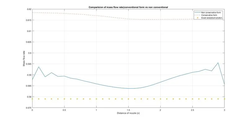
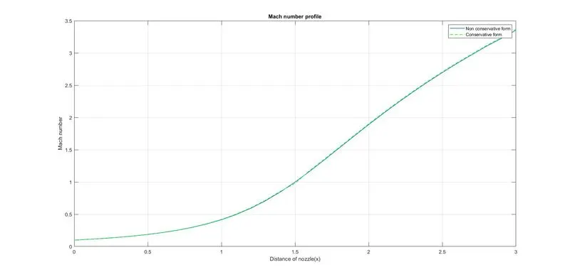
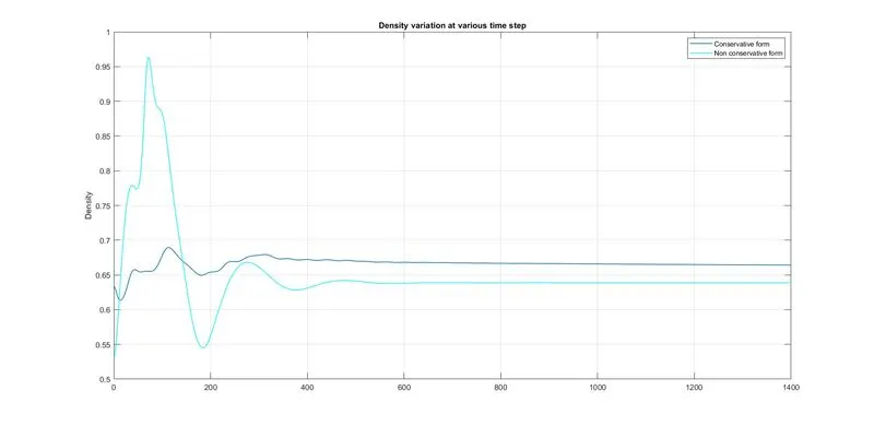
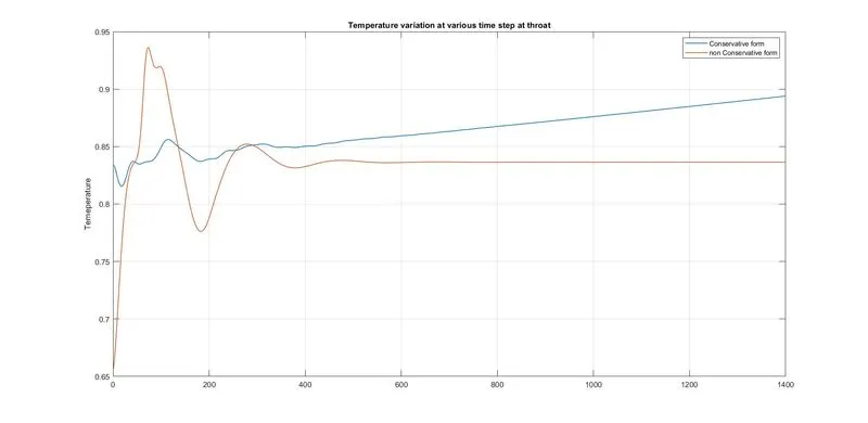
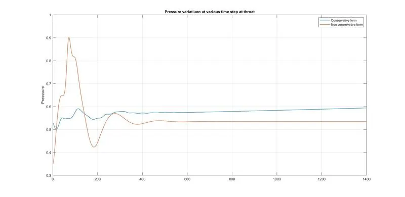
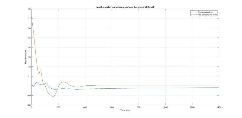
- Conservative form taking less time as comapred to non conservative form.
- The accuracy in case of non consevative form is more as comapared to conservative form.
- The conservative results are more accurate in mass flow rate whereas non conservative results are more accurate in primitive variables. However we can say that non conservative form has higher accuracy compared to conservative form.
- It is observed that as CFL value increases as the density, pressure and Temperature ratio increases. But however mach number decreases.
- The increase or decrease in CFL value doesnt effect the conservative form solution.