Week 7 - Simulation of a 1D Supersonic nozzle flow simulation using Macormack Method
Objective :
To simulate the isentropic flow through a quasi 1D subsonic-supersonic nozzle by deriving both conservative and non conservative forms of governing equation and solve them by using Macormack Method in matlab.
Problem statement :
- Need to determine the steady-state temperature distribution for the flow-field variables and to investigate the difference between the two forms of governing equations by comparing their solutions.
- To plot steady-state distribution of primitive variables inside the nozzle.
- To plot time-wise variation of the primitive variables.
- To plot variation of Mass flow rate distribution inside the nozzle at different time steps during the time-marching process.
- To plot comparison of Normalized mass flow rate distributions of both forms.
Theory :
Mach number :
It is a dimensionless quantity representing the ratio of flow velocity to the local speed of the sound.
M - Mach number.
u - Flow velocity.
c - Velocity of sound.
Nozzle diagram :
The nozzle has three main sections
1. convergent.
2. Throat.
3. Divergent
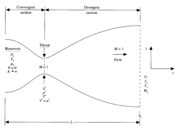
- At convergent section the flow velocity is less than the sound velocity therefore there mach number is less than 1.
- At throat section the flow velocity is equal to the sound velocity therefore there mach number is equal to 1.
- At divergent section the flow velocity is greater than the sound velocity therefore there mach number is greater than 1.
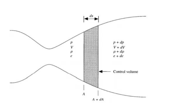
Program :
Main program :
clear all
close all
clc

% solving Quasi 1-D super sonic nozzle flow equations
% In put parameter
% No. of grid points
n=31;

gamma = 1.4
x=linspace(0,3,n);
dx = x(2)-x(1);

% No. of timeste
nt = 1400
% courant number
c = 0.5;

% function for non conservative form
tic;
[mass_flow_rate_nc, pressure_nc, mach_number_nc, rho, v, t, rho_throat_nc, v_throat_nc, temp_throat_nc, mass_flow_rate_throat_nc, pressure_throat_nc, mach_number_throat_nc] = non_conservative_form(x,dx,n,gamma,nt,c);
time = toc;
fprintf('Simulation time for non conservative form = %0.4f',time);
hold on

% plotting
% Timestep variation of properties at the throat area in non conservative
% form

figure(2)

%Density
subplot(4,1,1)
plot(rho_throat_nc,'color','r')
ylabel('Density')
legend({'Density at throat'});
axis([0 1400 0 max(rho_throat_nc)]);
grid minor;
title('Variation of field variables with respect to time step at throat area for non-conservative form')

% Temperature
subplot(4,1,2)
plot(temp_throat_nc,'color','c')
ylabel('Temperature')
legend({'Temperature at throat'});
axis([0 1400 0.6 max(temp_throat_nc)]);
grid minor;


% Pressure
subplot(4,1,3)
plot(pressure_throat_nc,'color','c')
ylabel('pressure')
legend({'pressure at throat'});
axis([0 1400 0.4 max(pressure_throat_nc)]);
grid minor;


% Mach number
subplot(4,1,4)
plot(mach_number_throat_nc,'color','r')
xlabel('Timesteps')
ylabel('pressure')
legend({'Mach number at throat'});
axis([0 1400 0.6 max(mach_number_throat_nc)]);
grid minor;


% Steady state simulation for primitive values for non conservative form
figure(3);

%Density

subplot(4,1,1)
plot(x,rho,'color','m')
ylabel('Densty')
legend({'Density'});
axis([0 3 0 max(rho)])
grid minor;
title('Variation of field variable along the length of nozzle for non-conservative form')

% Temperature
subplot(4,1,2)
plot(x,t,'color','c')
ylabel('Temperature')
legend({'Temperature'});
axis([0 3 0 max(t)])
grid minor;

% pressure
subplot(4,1,3)
plot(x,pressure_nc,'color','g')
ylabel('pressure')
legend({'pressure'});
axis([0 3 0 max(pressure_nc)])
grid minor;

% Mach number
subplot(4,1,4)
plot(x,mach_number_nc,'color','y')
ylabel('Mach Number')
legend({'Mach Number'});
axis([0 3 0 max(mach_number_nc)])
grid minor;

% function for conservative form
tic;
[mass_flow_rate_c, pressure_c, mach_number_c, rho_c, v_c, temp_c, rho_throat_c, v_throat_c, temp_throat_c, mass_flow_rate_throat_c, pressure_throat_c, mach_number_throat_c] = conservative_form(x,dx,n,gamma,nt,c);
time = toc;
fprintf('Simulation time for conservative form = %0.4f',time);
hold on

% plotting
% Timestep variation of properties at the throat area in conservative form

figure(5)

% Density
subplot(4,1,1)
plot(rho_throat_c,'color','m')
ylabel('Density')
legend({'Density at throat'});
axis([0 1400 0.5 max(rho_throat_c)]);
grid minor;
title('Variation of field variables with respect to time step at throat area for conservative form')

% Temperature
subplot(4,1,2)
plot(temp_throat_c,'color','c')
ylabel('Temperature')
legend({'Temperature at throat'});
axis([0 1400 0.8 max(temp_throat_c)]);
grid minor;


% Pressure
subplot(4,1,3)
plot(pressure_throat_c,'color','g')
ylabel('pressure')
legend({'pressure at throat'});
axis([0 1400 0.4 max(pressure_throat_c)]);
grid minor;

% Mach number
subplot(4,1,4)
plot(mach_number_throat_c,'color','y')
xlabel('Timesteps')
ylabel('Mach number')
legend({'Mach number at throat'});
axis([0 1400 0.9 max(mach_number_throat_c)]);
grid minor;

% Steady state simulation for primitive values for non conservative form
figure(6);

% Density
subplot(4,1,1)
plot(x,rho_c,'color','m')
ylabel('Density')
legend({'Density'});
axis([0 3 0 max(rho_c)])
grid minor;
title('Variation of flow rate distribution - conservative form')

% Temperature
subplot(4,1,2)
plot(x,temp_c,'color','c')
ylabel('Temperature')
legend({'Temperature'});
axis([0 3 0 max(temp_c)])
grid minor;

% pressure
subplot(4,1,3)
plot(x,pressure_c,'color','g')
ylabel('pressure')
legend({'pressure'});
axis([0 3 0 max(pressure_c)])
grid minor;

% Mach number
subplot(4,1,4)
plot(x,mach_number_c,'color','y')
xlabel('Nozzle length')
ylabel('Mach Number')
legend({'Mach Number'});
axis([0 3 0 max(mach_number_c)])
grid minor;

% Comparison plot of normalized mass flow rate of both forms
figure(7)
hold on
plot(x,mass_flow_rate_nc,'r','linewidth',1.25)
hold on
plot(x,mass_flow_rate_c,'b','linewidth',1.25)
hold on
grid on

legend('Non-conservative','Conservative');
xlabel('length of domain')
ylabel('mass flow rate')
title('Comparison of normalized mass flowrate of both forms')
Sub program :
Conservative form :
% Conservative form

function [mass_flow_rate_c, pressure_c, mach_number_c, rho_c, v_c, temp_c, rho_throat_c, v_throat_c, temp_throat_c, mass_flow_rate_throat_c, pressure_throat_c, mach_number_throat_c] = conservative_form(x,dx,n,gamma,nt,c)

% Determining initial profile of density or temperature
for i=1:n

    if (x(i) >=0 && x(i) <=0.5)
        rho_c(i) = 1;
        temp_c(i) = 1;
    elseif (x(i) >=0.5 && x(i) <= 1.5)
        rho_c(i) = 1-0.366*(x(i)-0.5);
        temp_c(i) = 1 - 0.167*(x(i)-0.5);
    elseif (x(i) >=1.5 && x(i) <= 3)
        rho_c(i) = 0.634-0.3879*(x(i)-1.5);
        temp_c(i) = 0.833 - 0.3507*(x(i)-1.5);
    end
end


a = 1+2.2*(x-1.5).^2;
throat = find(a==1);

% Calculate initial profiles
v_c = 0.59./(rho_c.*a);
pressure_c = rho_c.*temp_c;

%Calculate the initial solution vectors(U)
U1 = rho_c.*a;
U2 = U1.*v_c;
U3 = U1.*((temp_c./(gamma-1))+(gamma/2).*(v_c.^2));

% Outer time loop
for k =1:nt
    % Time-step control
    dt = min(c.*dx./(sqrt(temp_c) + v_c));
%     Dt = temp_c.^0.5;
%     dt = min(c*(dx./(Dt + v_c)));


    %saving a copy of old values
    U1_old = U1;
    U2_old = U2;
    U3_old = U3;

    %Calculating the flux vector(F)
    F1 = U2;
    F21 = (U2.^2)./(U1);
    F22 = (gamma-1)/(gamma);
    F23 = U3 - ((gamma/2).*F21);
    F2 = F21 + F22 * F23;


    F31 = (U2.*U3)./(U1);
    F32 = (gamma*(gamma-1))/2;
    F33 = (U2.^3)./(U1.^2);
    F3 = gamma.*F31 - (F32.*F33);


    % predictor method
    for j= 2:n-1

        % Calculating the source term(J)
        J2_P(j) = (1/gamma)*(rho_c(j)*temp_c(j))*((a(j+1)-a(j))/dx);

        % continuity equation
        dU1_dt_P(j) = -((F1(j+1)- F1(j))/dx);

        % Momentum equation
        dU2_dt_P(j) = -((F2(j+1)- F2(j))/dx)+J2_P(j);

        % Energy Equation
        dU3_dt_P(j) = -((F3(j+1) - F3(j))/dx);


        % Updating new values
        U1(j) = U1(j)+ dU1_dt_P(j)*dt;
        U2(j) = U2(j)+ dU2_dt_P(j)*dt;
        U3(j) = U3(j)+ dU3_dt_P(j)*dt;

    end

    % Updating flux vectors
    rho_c =  U1./a;
    v_c = U2./U1;
    temp_c = (gamma-1)*((U3./U1 - (gamma/2)*(v_c).^2));

     %Calculating the flux vector(F)
    F1 = U2;
    F21 = (U2.^2)./(U1);
    F22 = (gamma-1)/(gamma);
    F23 = U3 - ((gamma/2).*F21);
    F2 = F21 + F22 * F23;


    F31 = (U2.*U3)./(U1);
    F32 = (gamma*(gamma-1))/2;
    F33 = (U2.^3)./(U1.^2);
    F3 = gamma.*F31 - (F32.*F33);


    %corrector Method
    for j = 2:n-1

        % updating the source term(J)
        J2(j) = (1/gamma)*rho_c(j)*temp_c(j)*((a(j)-a(j-1))/dx);

        %Simplifying the Equation's spatial terms
        dU1_dt_C(j) = -((F1(j)-F1(j-1))/dx);
        dU2_dt_C(j) = -((F2(j)-F2(j-1))/dx)+J2(j);
        dU3_dt_C(j) = -((F3(j)-F3(j-1))/dx);
    end

    % Compute Average time derivative
    dU1_dt = 0.5*( dU1_dt_P +  dU1_dt_C);
    dU2_dt = 0.5*( dU2_dt_P +  dU2_dt_C);
    dU3_dt = 0.5*( dU3_dt_P +  dU3_dt_C);

    % Final solution update
    for i = 2:n-1
        U1(i) = U1_old(i) + dU1_dt(i)*dt;
        U2(i) = U2_old(i) + dU2_dt(i)*dt;
        U3(i) = U3_old(i) + dU3_dt(i)*dt;
    end

    % Applying Boundary conditions
    % At Inlet
    U1(1) = rho_c(1)*a(1);
    U2(1) = 2*U2(2)-U2(3);

    v_c(1) = U2(1)./U1(1);
    U3(1) = U1(1)*((temp_c(1)/(gamma-1))+((gamma/2)*(v_c(1)).^2));

    % At Outlet
    U1(n) = 2*U1(n-1)-U1(n-2);
    U2(n) = 2*U2(n-1)-U2(n-2);
    U3(n) = 2*U3(n-1)-U3(n-2);
    % Final primitive value update
    rho_c =  U1./a;
    v_c = U2./U1;
    temp_c = (gamma-1)*((U3./U1 - (gamma/2)*(v_c).^2));

    % Defining Mass flow rate, pressure and Mach number

    mass_flow_rate_c = rho_c.*a.*v_c;
    pressure_c = rho_c.*temp_c;
    mach_number_c = (v_c./sqrt(temp_c));

    % Calculating Variables at throat section
    rho_throat_c(k) = rho_c(throat);
    temp_throat_c(k) = temp_c(throat);
    v_throat_c(k) = v_c(throat);
    mass_flow_rate_throat_c(k) = mass_flow_rate_c(throat);
    pressure_throat_c(k) = pressure_c(throat);
    mach_number_throat_c(k) = mach_number_c(throat);

    % plotting
    % comparison of non-dimensional mass flow rates at diferent time
    % steps

    figure(8)
    if k==50
        plot(x, mass_flow_rate_c,'m','linewidth',1.25);
        hold on
    elseif k == 100
        plot(x, mass_flow_rate_c,'c','linewidth',1.25);
        hold on
    elseif k == 200
        plot(x, mass_flow_rate_c,'g','linewidth',1.25);
        hold on
    elseif k == 400
        plot(x, mass_flow_rate_c,'y','linewidth',1.25);
        hold on
    elseif k == 800
        plot(x, mass_flow_rate_c,'k','linewidth',1.25);
       hold on
    end

    % Labelling
    title('Mass flow rates at different timesteps - conservative form')
    xlabel('Distance')
    ylabel('Mass flow rate')
    legend({'50th Timestep','100th Timestep','200th Timestep','400th Timestep','800th Timestep'})
    axis([0 3 0.4 1])
    grid on

    end
end
Non-conservative form :
function [mass_flow_rate_nc, pressure_nc, mach_number_nc, rho, v, t, rho_throat_nc, v_throat_nc, temp_throat_nc, mass_flow_rate_throat_nc, pressure_throat_nc, mach_number_throat_nc] = non_conservative_form(x,dx,n,gamma,nt,c);

% Calculate initial profiles
rho = 1-0.3146*x;
t = 1-0.2314*x;              % t is a temperature
v = (0.1+1.09*x).*t.^(1/2);

% Area
a = 1+2.2*(x-1.5).^2;
throat = find(a==1)

% outer time loop
for k=1:nt

    %Time step control
    dt = min(c.*dx./(sqrt(t) + v));

    % Saving a copy of old values
    rho_old = rho;
    v_old = v;
    t_old = t;

    % predictor method
    for j = 2:n-1
        dvdx = (v(j+1)-v(j))/(dx);
        drhodx = (rho(j+1)-rho(j))/(dx);
        dtdx = (t(j+1)-t(j))/(dx);
        dlogadx = (log(a(j+1))-log(a(j)))/(dx);

        %continuity equation
        drhodt_p(j) = -rho(j)*dvdx - rho(j)*v(j)*dlogadx-v(j)*drhodx;

        %momentum equation
        dvdt_p(j) = -v(j)*dvdx - (1/gamma)*(dtdx+(t(j)/rho(j))*drhodx);

        % Energy equation
        dtdt_p(j) = -v(j)*dtdx -(gamma-1)*t(j)*(dvdx + v(j)*dlogadx);

        %solution update
        rho(j) = rho(j)+drhodt_p(j)*dt;
        v(j) = v(j)+dvdt_p(j)*dt;
        t(j) = t(j)+dtdt_p(j)*dt;
    end

     % corrector method
    for j = 2:n-1
        dvdx = (v(j)-v(j-1))/(dx);
        drhodx = (rho(j)-rho(j-1))/(dx);
        dtdx = (t(j)-t(j-1))/(dx);
        dlogadx = (log(a(j))-log(a(j-1)))/(dx);

        %continuity equation
        drhodt_c(j) = -rho(j)*dvdx - rho(j)*v(j)*dlogadx-v(j)*drhodx;

        %momentum equation
        dvdt_c(j) = -v(j)*dvdx - (1/gamma)*(dtdx+(t(j)/rho(j))*drhodx);

        % Energy equation
        dtdt_c(j) = -v(j)*dtdx -(gamma-1)*t(j)*(dvdx + v(j)*dlogadx);

    end

    % compute the average time derivation
    drhodt = 0.5*(drhodt_p + drhodt_c);
    dvdt = 0.5*(dvdt_p + dvdt_c);
    dtdt = 0.5*(dtdt_p + dtdt_c);

    % Final solution update
    for i=2:n-1
       v(i) = v_old(i) +dvdt(i)*dt;
       rho(i) = rho_old(i) +drhodt(i)*dt;
       t(i) = t_old(i)+dtdt(i)*dt;
    end

    %Apply boundary conditions
    % Inlet
    v(1) = 2*v(2) - v(3);

    %Outlet
    v(n) = 2*v(n-1)- v(n-2);
    rho(n) = 2*rho(n-1)- rho(n-2);
    t(n) = 2*t(n-1)- t(n-2);


    % Defining Mass flow rate, pressure and Mach number

    mass_flow_rate_nc = rho.*a.*v;
    pressure_nc = rho.*t;
    mach_number_nc = (v./sqrt(t));

    % Calculating Variables at throat section
    rho_throat_nc(k) = rho(throat);
    temp_throat_nc(k) = t(throat);
    v_throat_nc(k) = v(throat);
    mass_flow_rate_throat_nc(k) = mass_flow_rate_nc(throat);
    pressure_throat_nc(k) = pressure_nc(throat);
    mach_number_throat_nc(k) = mach_number_nc(throat);

    % plotting
    % comparison of non-dimensional mass flow rates at diferent time
    % steps

    figure(4)
    if k==50
        plot(x, mass_flow_rate_nc,'m','linewidth',1.25);
        hold on
    elseif k == 100
        plot(x, mass_flow_rate_nc,'c','linewidth',1.25);
        hold on
    elseif k == 200
        plot(x, mass_flow_rate_nc,'g','linewidth',1.25);
        hold on
    elseif k == 400
        plot(x, mass_flow_rate_nc,'y','linewidth',1.25);
        hold on
    elseif k == 800
        plot(x, mass_flow_rate_nc,'k','linewidth',1.25);
        hold on
    end

    % Labelling
    title('Mass flow rates at different timesteps - non-conservative form')
    xlabel('Distance')
    ylabel('Mass flow rate')
    legend({'50th Timestep','100th Timestep','200th Timestep','400th Timestep','800th Timestep'})
    axis([0 3 0 2])
    grid on

end
Output :
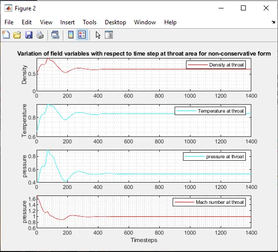
The variation of flow field variables at throat section with respect to time step for non-conservative form as shown above. From the graph it is clear that the flow field variables are almost reached the steady state solution after the 400th iteration.
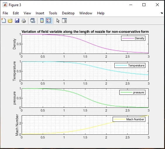
The above graph shows that the variation of flow field varialbles along the length of the nozzle for the non conservative form. In the above graph it is clear that the flow field variables such as density, pressure, temperature decreases and mach number increases with a increase in length of the nozzle.
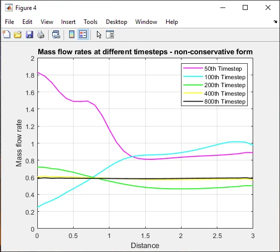
The above figure shows that the variation of mass flow rate with respect to time step for non-conservation form. From the graph it is clear that the mass flow rate is almost stable after the 400th time step.
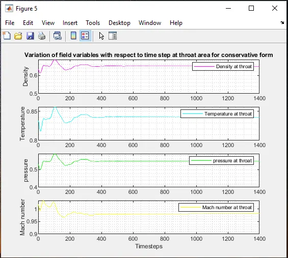
The variation of flow field variables at throat section with respect to time step for conservative form as shown above. From the graph it is clear that the flow field variables are almost reached the steady state solution after the 400th iteration.
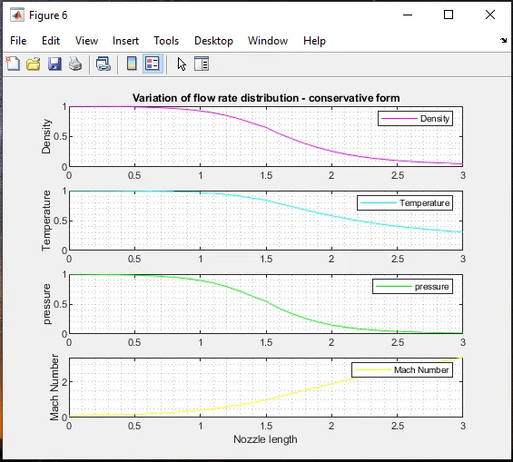
The above graph shows that the variation of flow field varialbles along the length of the nozzle for the conservative form. In the above graph it is clear that the flow field variables such as density, pressure, temperature decreases and mach number increases with a increase in length of the nozzle.
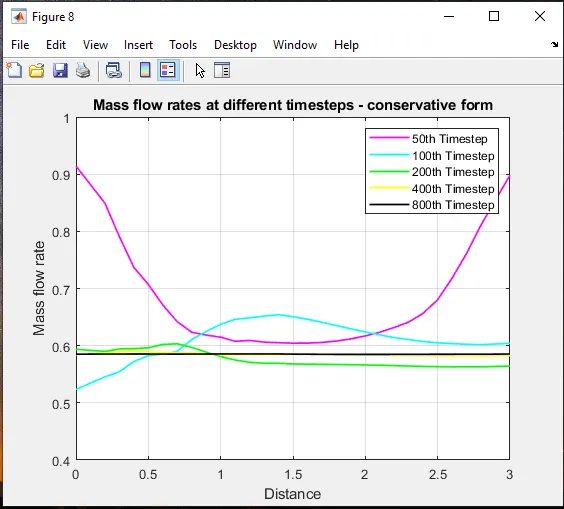
The above figure shows that the variation of mass flow rate with respect to time step for conservation form. From the graph it is clear that the mass flow rate is almost stable after the 400th time step.
Normalized mass flow rate distributions of both forms :
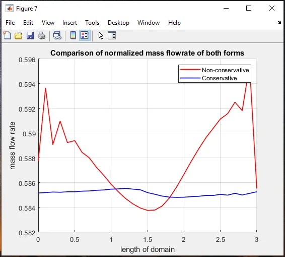
The above figure shows that the variation of mass flow rate at the both the forms. From the graph it is clear that the mass flow rate of conservative forms produces a stable result when compare to that of non conservative form. We can also find that the mass flow rate is minimum at the throat then it expands in the non conservative form. From figure the average mass flow rate of conservative form is 0.585
Grid dependence test :
In order to conduct grid dependency test for the flow field variables at the throat setion at the end of 1400th time step the solutions at two conditions need to be considered one with 31 grid points and the other with 61 grid points.
| GRID DEPENDENCE TEST | |||||
| Type of Form | No. of Grids(n) | Primitive variables | |||
| Density | Pressure | Temperature | Mach Number | ||
| Non Conservative from | 31 | 0.6387 | 0.5342 | 0.8365 | 0.9994 |
| 61 | 0.6376 | 0.5326 | 0.8354 | 0.9997 | |
| Conservative form | 31 | 0.6504 | 0.5463 | 0.8400 | 0.9818 |
| 61 | 0.6383 | 0.5330 | 0.8351 | 0.9993 | |
| Expected output | 0.634 | 0.528 | 0.833 | 1 | |
From the table it is clear that the solution of 61 grid points almost equal to the exact solution when compare to that of the solution of 31 grid points. More the number of grid points more will the computational time but at the same time we can able to produce the accurate result than the lesser grid point.
Conclusion :
Simulation of isentropic flow through a quasi 1D subsonic-supersonic nozzle by deriving both conservative and non conservative forms of governing equation and solve them by using Macormack Method in matlab is successfully compiled and the results are discussed at the output. Between conservative and non-conservative forms, In order to get a smooth solution conservative form is preferred because non-conservative form may leads to shocks at the shock flow region.