Week 7 - Simulation of a 1D Supersonic nozzle flow simulation using Macormack Method

            INTRODUCTION TO THE GIVEN PROBLEM

We consider the steady isoentropic flow through the convergent -divergent nozzle as given in diagram below.

   

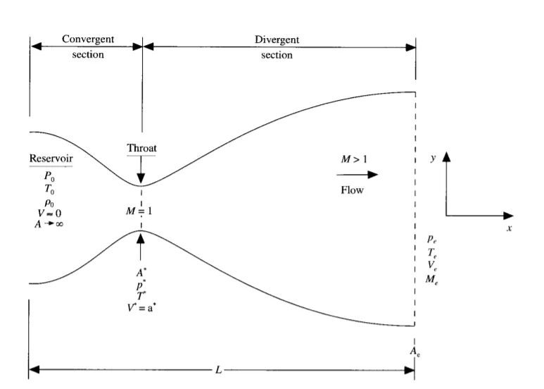
The flow at the inlet to the nozzle comes from the reservoir is large (therotically A→∞">A→∞0 and hence the velocity is very small (V→0)">(V→0) .Thus ,po">po and To">To are the stagnantation values or total pressure and total temperature,respectively.The flow expands isoentropically to supersonic speeds at the nozzle exit,where the exit pressure,temperature where exit parameters are reperesented with subscript e.

The flow is locally subsonic in the convergent section of the nozzle,sonic at the throat (minimum area) ,and supersonic at the divergent section . The sonic flow (M=1)at  the throat means the local velocity at this section is equal to the local speed of the sound.We can repersent the throat values with our own representation either with * or any other.

(AA∗)2=1M2⋅(2γ+1⋅(1+γ-12⋅M2))γ+1γ-1">(A/A∗)^2=1/M^2⋅(2/γ+1⋅(1+γ−1/2⋅M^2))(γ+1)/(γ−1)

`here γ">γ is the ratio of specific heat.For air at standard conditons it is equal to 1.4`

Some other equations include 

(ppo)=(1+γ-12⋅M2)-γγ-1">(p/po)=(1+(γ−1)/2⋅M^2)−(γ/γ−1)

(ρρo)=(1+γ-12⋅M2)-1γ-1">(ρ/ρo)=(1+(γ−1)/2⋅M^2)−(1/γ−1)

(TTo)=(1+γ-12⋅M2)-1">(T/To)=(1+(γ−1)/2⋅M^2)−1

Mach number  is a dimensionless quantity in fluid dynamics representing the ratio of flow velocity past a boundry to the local speed of sound

       M=uc,">M=u/c,,

where:

M  is the local Mach number,

u  is the local flow velocity with respect to the boundaries (either internal, such as an object immersed in the flow, or external, like a channel), and

c  is the speed of sound in the medium, which in air varies with the square root of the thermodynamics temeprature.

Assuming air to be an ideal gas, the formula to compute Mach number in a subsonic compressible flow is derived from Bernoullis equation for M < 1:

M=2γ+1⋅[(qcp+1)γ-1γ-1]">M=2/(γ+1)⋅⎡((q/cp)+1)(γ−1)/(γ−1)⎤

and the  speed of sound varies with teperature as follows:

c=γ⋅R∗T">c=√γ⋅R∗T

whereqc">qc is imact pressure

p">p is the static pressure.

γ">γ is the ratio of specific heat of a gas at a constant pressure to heat at a constant volume (1.4 of air).

R∗">R is the specific gas constant.

Set Up

MaCcormack mathod:

In computational fluid dynamics, the MacCormack method is a widely used discretization scheme for the numerical solution of hyperbolic partial differential equations.

Maccormacks method provides second order accuracy without the invlovement of second order derivative thus reducing the complexity  of the calculation.It is a explicit method.

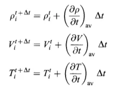
According to Maccormacks method  the value of variable at grid point i,j at time t+dt is given as follows:

Factual=FInitial+∂(f)(∂t)avg⋅∂t">Factual=FInitial+∂(f)/(∂t)avg⋅∂t

The average time derivative can be found as follows ,which is the  half of sum of predicotor value and correcotr value .

(∂v∂t)avg=(∂v∂t)p+(∂v∂t)c">(∂v/∂t)avg=(∂v/∂t)p+(∂v/∂t)c

So basically before that we need to set up equations for solving the predictor and corrector method.

Governing equations:

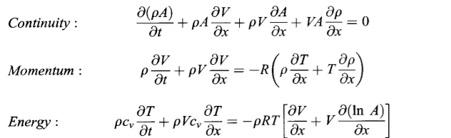
The super sonic flow through nozzle is governed by Navier stokes equations,which could be derived for both the cases of conservative and Non conservative methods.

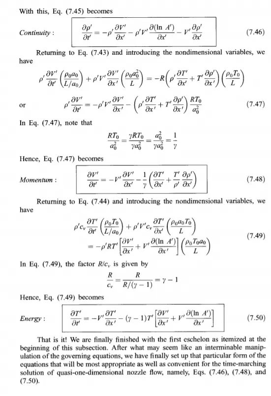
The continuity equation can be given as follows:

∂ρ′∂t′=-(ρ′)⋅∂V′∂x′-ρ′⋅V′⋅∂(lnA′)∂x′-V′⋅(∂ρ′∂x′)">∂ρ′/∂t′=−(ρ′)⋅∂V′/∂x′−ρ′⋅V′⋅∂(lnA′)/∂x'−V′⋅(∂ρ′/∂x′)

The momentum equation:

∂V′(∂t)′=-V′⋅∂V′∂x′-1γ⋅(∂T′∂x′+T′ρ′⋅∂ρ′∂x′)">∂V′/(∂t)′=−V′⋅∂V/∂x′−1/γ⋅(∂T′/∂x′+T′/ρ′⋅∂ρ′/∂x′)

The energy equation is as follows:

∂T′∂t′=-V′⋅∂T′∂x′-(γ-1)⋅T′⋅[∂V′∂x′+V′⋅∂(lnA′)∂x′]">∂T′/∂t′=−V′⋅∂T′/∂x′−(γ−1)⋅T′⋅[∂V′/∂x′+V′⋅∂(lnA′)/∂x

These equation can be derived from the 

The To">To and ρo">ρo arethe reservoir temperature and density.We define the non dimensional temperature and density respectively as follows:

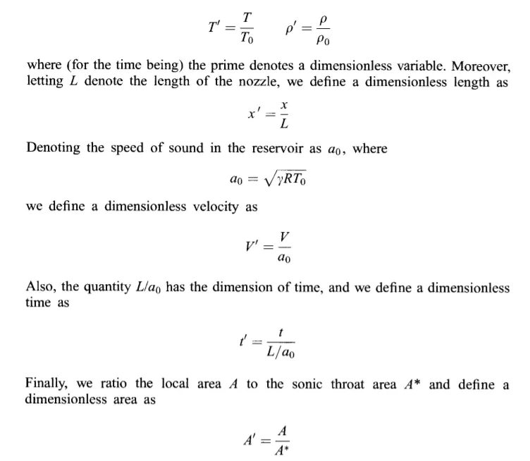
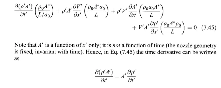
Next we define the initial condition :

• The shape of nozzle ,A=A( x) is specified and held fixed ,independent of time,For this case we take the parabolic area distribution 
• A=1+2.2⋅(x-1.5)2">A=1+2.2⋅(x−1.5)^2    0≤x≤3">0≤x≤30≤3
• For density ,Temperature and velocity is given by
• ρ=1-0.3146⋅x">ρ=1−0.3146⋅x
• T=1-0.2314x">T=1−0.2314x
• V=(0.1+1.09x)⋅T">V=(0.1+1.09x)⋅√T
• Pressure  P=ρ⋅T">P=ρ⋅T
• Mach number= uT">u√T
• The above mentioned are the initial conditions at t=0

Next we come to predictor step:

This is a kind of descritisation step.Where we descretize with forward difference equation.

We first set up the finite difference expressions as follows:

We set up the spatial derivatives as forward differences .Also to reduce the complexity of the notation we will drop the prime to denote the dimensionless variable.

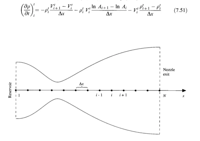
And some of the other equations including for other variables like momentum and energy as well  .

For grid generation we  divide the length of the nozzle in number of points along the axis .The characteristics of the flow changes from subsonic to super sonic from right to left .The distance between the two grid points is dx.Smaller the mesh size the error also decreases.

In discretisation part we apply thr MaCcormach technique to solve the the conservative and non conservative forms of governing equations.

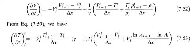
From these we get the predicted equation as follows: These are denoted by barred quantities.

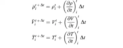
`n these equations ρit,Vit">ρti,Vti and Tit">Tti are the known values at tim`

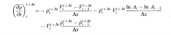
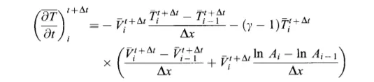
Next step is  the corrcetor method:

Here we use the backward differencing scheme and rest remains same as that of the predictor method.

Continuity equation

Momentum equation

Energy equation

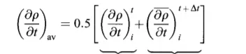
Calculation of Average:

Its basically the half of the sum of corrector and predictor value.

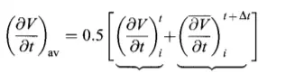
Then finally the corrected values at time t+ Δt">ΔtΔare:

Calculation of time step:

dt=C⋅dxu+a">dt=C⋅dx/(u+a)

where  C is the courant number itts value is 0.5

u is the local velocity 

a is the local speed of sound

Boundry condtions at subsonic section

 By using linear extrapolation 

V1=2⋅V2-V3">V1=2⋅V2−V3

Density and Temperature at point  1 is held fixed.

Supersonic outflow boundry conditions:

VN=2⋅VN-1-VN-2">VN=2⋅VN−1−VN−2

ρN=2⋅ρN-1-ρN-2">ρN=2⋅ρN−1−ρN−2

TN=2⋅TN-1-TN-2">TN=2⋅TN−1−TN−2

Conservative form

The equations  in  Conservative form in dimension less form is given as follows:

The continuity Equation:

• ∂(ρ′A′)∂t′+∂(ρ′A′V′)∂x′=0">∂(ρ′A′)/∂t′+∂(ρ′A′V′)/∂x′=0

The momentum equation

The energy equation :

The above are the non dimensional conservation form of the coninuity ,momentum and energy equations for quasi-one -dimensional flow ,respectively.The equations for quasi one dimensional flow can be expressed in generic form.Let us define the elements of the solution vector U ,flux vector F and the source term J as follows 

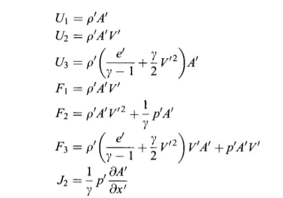
From the above equations we can write that 

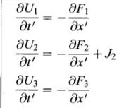
These are the equations we wish to  solve numerically by using the MacCormacks technique.

To obtain the primitve variables we must decode the elements U1,U2,U3 as follows.From the defination of U1,U2 and U3 given above we have 

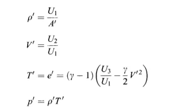
Expressing the flux and source term in form of solution  vectors

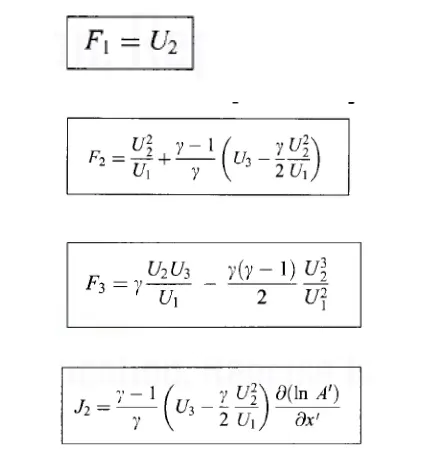
Applying the boundry conditions:

Inlet boundry conditions:

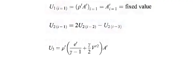
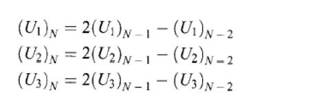
Outlet boundry condition:The flow properties at the downstream ,supersonic outflow boundry are obtained by linear extrapolation from the two adjacent internal points.

If N denotes the grid point at the outflow boundry ,then:

The values of  F1,F2 and F3 at grid point i=N  are obtained from the values of U1,U2 and U3 at point i=N using the equations.

Initial conditions:

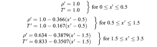
We can set this condition  by using the if statements.

The code for the above:

close all
clear all
clc

%input parameters 
n=31;
x=linspace(0,3,n);
dx=x(2)-x(1);
gamma=1.4;
CFL=0.5;
Area=1+2.2*(x-1.5).^2;
throat=((n+1)/2);
nt=1400;

%main body
tic;
[V,rho,T,m,M,P,V_t,rho_t,T_t,m_t,M_t,P_t]=non_conservative(throat,x,gamma,dx,Area,n,nt,CFL);
non_conservative=toc;

tic
[Vc,rhoc,Tc,cons_mass_flow_throat,Mc,pc,Vc_throat,rho_throat,T_throat,cons_mass_flow,Mc_throat,pc_throat]=conservative(throat,x,gamma,dx,Area,n,nt,CFL);
conservative=toc;

%plotting section 
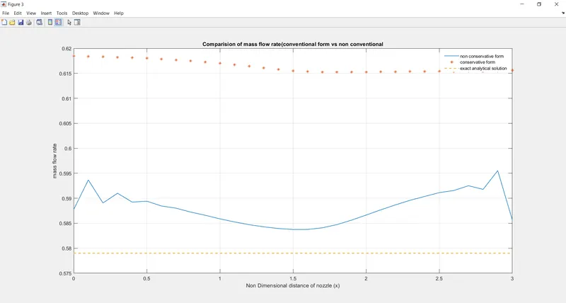
figure(3)
plot(x,m,'linewidth',0.95);
hold on;
plot(x,cons_mass_flow,'*');
%exact analytical solution rho*A*v=0.579
plot(x,linspace(0.579,0.579,n),'--','linewidth',1.5);
xlabel('Non Dimensional distance of nozzle (x)');
ylabel('mass flow rate');
legend('non conservative form','conservative form','exact analytical solution');
title('Comparision of mass flow rate(conventional form vs non conventional');
grid on ;

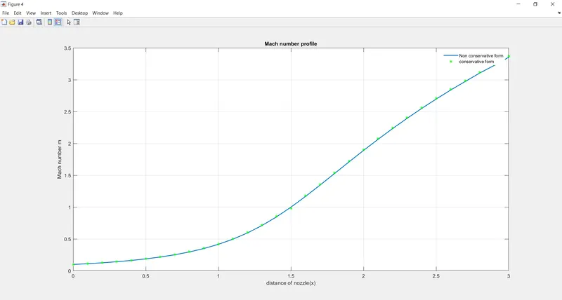
figure(4)
plot(x,M,'linewidth',1.5);
hold on
plot(x,Mc,'*','linewidth',0.65,'color','g');
grid on 
xlabel('distance of nozzle(x)');
ylabel('Mach number m');
legend('Non conservative form','conservative form');
title('Mach number profile');
grid on 
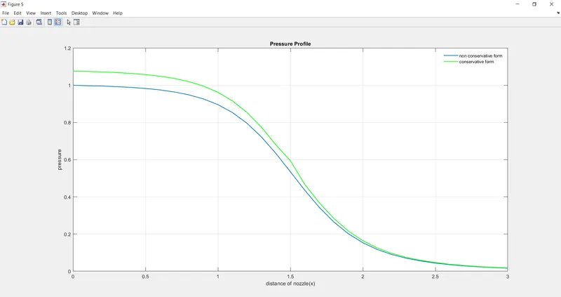
figure(5)

plot(x,P,'linewidth',1.25);
hold on 
plot(x,pc,'g','linewidth',1.25);
grid on 
xlabel('distance of nozzle(x)');
ylabel('pressure');
legend('non conservative form','conservative form');
title('Pressure Profile');
grid on 

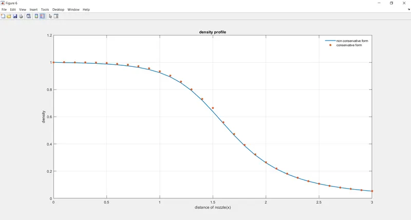
figure(6)
plot(x,rho,'linewidth',1.5)
hold on 

plot(x,rhoc,'*','linewidth',1.25);
grid on 
xlabel('distance of nozzle(x)');
ylabel('density');
legend('non conservative form','conservative form');
title('density profile');
grid on 
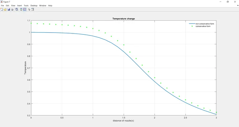
figure(7)

plot(x,T,'linewidth',1.5);
hold on 
plot(x,Tc,'*','linewidth',0.65,'color','g');
grid on
xlabel('distance of nozzle(x) ');
ylabel('Temperature');
legend('non conservative form','conservative form');
title('Temperature change');

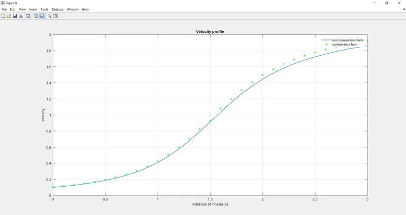
figure(8)
plot(x,V,'linewidth',1.0);
hold on ;
plot(x,Vc,'*','linewidth',0.65,'color','g');
grid on 
xlabel('distance of nozzle(x)');
ylabel('velocity');
legend('non conservative form','conservative form');
title('Velocity profile');

grid on

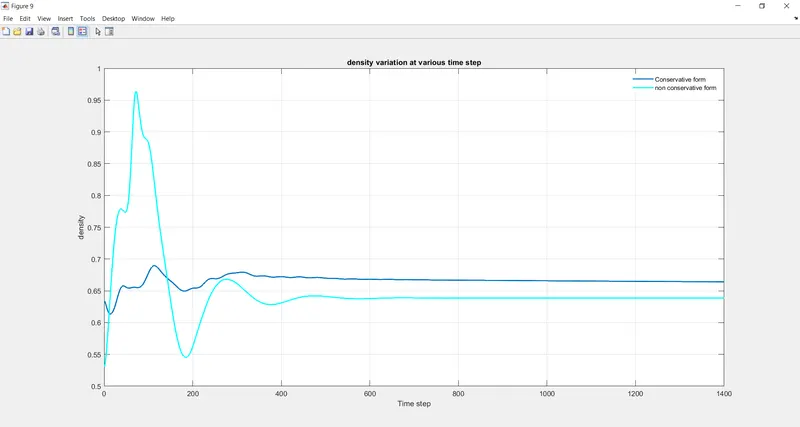
figure(9)

plot(1:nt,rho_throat,'linewidth',1.5);
hold on 
plot(1:nt,rho_t,'c','linewidth',1.65);
grid on 
ylabel('density');
legend('Conservative form','non conservative form');
title('density variation at various time step');
grid on 

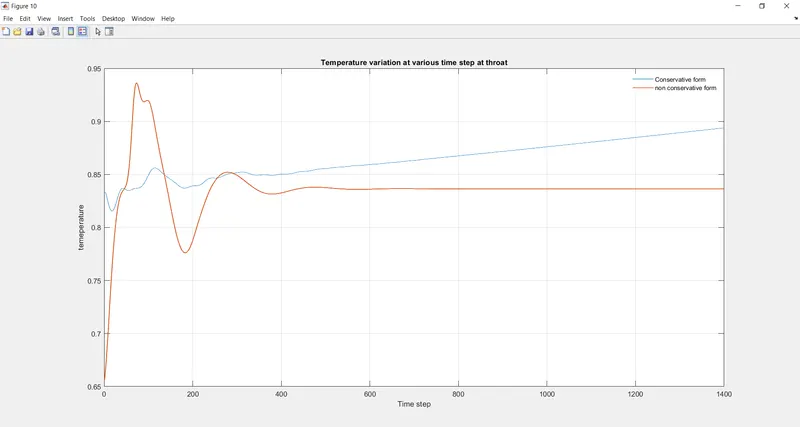
figure(10)
plot(1:nt,T_throat,'linewidth',0.75);
hold on 
plot(1:nt,T_t,'linewidth',0.95)
grid on 
ylabel('temeperature');
legend('Conservative form','non conservative form');
title('Temperature variation at various time step at throat');
grid on 


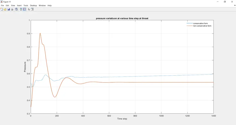
figure(11)

plot(1:nt,pc_throat,'linewidth',0.85)
hold on 
plot(1:nt,P_t,'linewidth',0.95)
grid on 
ylabel('Presssure');
legend('conservative form','non conservative form');
title('pressure variatiuon at various time step at throat');
grid on

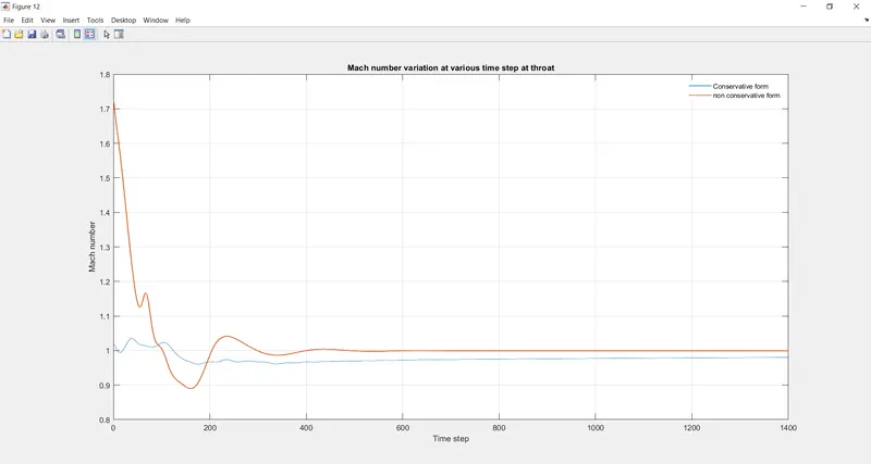
figure(12)
plot(1:nt,Mc_throat,'linewidth',0.85);
hold on 
plot(1:nt,M_t,'linewidth',0.90)
grid on 
xlabel('Time step');
ylabel('Mach number');
legend('Conservative form','non conservative form');
title('Mach number variation at various time step at throat');

%function for non-conservative form 

function [V,rho,T,m,M,P,V_t,rho_t,T_t,m_t,M_t,P_t]=non_conservative(throat,x,gamma,dx,A,n,nt,C)
  
%calculations

rho =1-0.3146*x;
T=1-0.2314*x;
V=(0.1+1.09*x).*T.^0.5;

dt=min(C.*(dx./(sqrt(T)+V)));

for it=1:nt
    rho_old=rho;
    V_old=V;
    T_old=T;
    
    for j=2:n-1
        
        drhodx_p=(rho(j+1)-rho(j))/dx;
        dvdx_p=(V(j+1)-V(j))/dx;
        dtdx_p=(T(j+1)-T(j))/dx;
        dlogA_dx_p=(log(A(j+1))-log(A(j)))/dx;
        
        %continuity equation
        drhodt_p(j)=-rho(j)*dvdx_p-rho(j)*V(j)*dlogA_dx_p-V(j)*drhodx_p;
        %momentum equation
        dvdt_p(j)=-V(j)*dvdx_p-(1/gamma)*(dtdx_p+(T(j)/rho(j))*drhodx_p);
        %energy equation
        dtdt_p(j)=-V(j)*dtdx_p-(gamma-1)*T(j)*(dvdx_p+V(j)*dlogA_dx_p);
        %solution update
        rho(j)=rho(j)+(drhodt_p(j))*dt;
        V(j)=V(j)+dvdt_p(j)*dt;
        T(j)=T(j)+dtdt_p(j)*dt;
    end
    
    %corrector step.
    for j=2:n-1
        drhodx_c=(rho(j)-rho(j-1))/dx;
        dvdx_c=(V(j)-V(j-1))/dx;
        dtdx_c=(T(j)-T(j-1))/dx;
        dlogA_dx_c=(log(A(j))-log(A(j-1)))/dx;
        
        %continuity equation
        drhodt_c(j)=-(rho(j)*dvdx_c)-rho(j)*V(j)*dlogA_dx_c-V(j)*drhodx_c;
        %momentum equation       
        dvdt_c(j)=-(V(j)*dvdx_c)-(1/gamma)*(dtdx_c+(T(j)/rho(j))*drhodx_c);
        %energy equation
        dtdt_c(j)=-(V(j)*dtdx_c)-(gamma-1)*T(j)*(dvdx_c+V(j)*dlogA_dx_c);
    end
        
    %average values
       dvdt=0.5*(dvdt_c+dvdt_p);
       drhodt=0.5*(drhodt_p+drhodt_c);
       dtdt=0.5*(dtdt_c + dtdt_p);
       
       for i=2:n-1
           rho(i)=rho_old(i)+drhodt(i)*dt;
           V(i)=V_old(i)+dvdt(i)*dt;
           T(i) = T_old(i)+dtdt(i)*dt;
       end
       V(1)=2*V(2)-V(3);
       V(n)=2*V(n-1)-V(n-2);
       rho(n) = 2*rho(n-1)-rho(n-2);
       T(n)=2*T(n-1)-T(n-2);
       
       m=rho.*A.*V;
       P=rho.*T;
       M=V./sqrt(T);
       
       
       rho_t(it)=rho(throat);
       V_t(it)=V(throat);
       T_t(it)=T(throat);
       P_t(it)=P(throat);
       M_t(it)=M(throat);
       m_t(it)=m(throat);
       
       rho_exact=0.634*ones(1,1400);
       t_exact=0.833*ones(1,1400);
       p_exact = 0.528*ones(1,1400);
       mach_exact=1*ones(1,1400);
      
       figure(1) 
       if it==50
           plot(x,m,'b','linewidth',1.5);
           hold on
        elseif it==100
              plot(x,m,'r','linewidth',1.5);
              hold on 
        elseif it==150
               plot(x,m,'c','linewidth',1.5);
               hold on 
        elseif  it==300
                plot(x,m,'g','linewidth',1.5);
                hold on 
        elseif  it==600
                plot(x,m,'y','linewidth',1.5);
                hold on 
        elseif it==900
                plot(x,m,'k','linewidth',1.5);
                hold on 
        elseif it==1400
                plot(x,m,'m','linewidth',1.5);
                grid on
       end
end

  xlabel('Non dimensional distance through nozzle (x)','fontsize',10);
  ylabel('Non dimensional mass flow rate through nozzle x','fontsize',10);
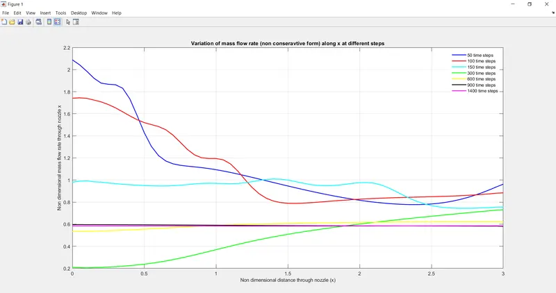
  title('Variation of mass flow rate (non conseravtive form) along x at different steps');
  legend({'50 time steps','100 time steps','150 time steps','300 time steps','600 time steps','900 time steps','1400 time steps'});
     
       
end

%conservative form
function [Vc,rhoc,Tc,cons_mass_flow_throat,Mc,pc,Vc_throat,rho_throat,T_throat,cons_mass_flow,Mc_throat,pc_throat]=conservative(throat,x,gamma,dx,A,n,nt,C)

R=8.314;
for i=1:n
    if (x(i)<=0.5)
        rho_in (i)=1;
        T_in(i)=1;
    elseif (x(i)>=0.5) && (x(i) <= 1.5)
            rho_in(i)=1-(0.366*(x(i)-0.5));
            T_in(i)=1-0.167*(x(i)-0.5);
        else 
                rho_in(i)=0.634-0.3879*(x(i)-1.5);
                T_in(i)=0.833-0.3507*(x(i)-1.5);
    end
end

 u_in=0.59./(rho_in.*A);
 rhoc = rho_in;
 Tc=T_in;
 Vc=u_in;
        
    



dt=0.0206;
t_sim=(nt-1)*dt;
t=0:dt:t_sim;

U1=rhoc.*A;
U2=rhoc.*A.*Vc;
U3=rhoc.*A.*((Tc/(gamma-1))+(0.5*gamma.*Vc.*Vc));

%Macormack method
for j=1:length(t)
    U1_old=U1;
    U2_old=U2;
    U3_old=U3;
    
    F1=U2;
    F2=((U2.^2)./U1)+((gamma-1)/gamma).*(U3-((gamma/2)*(U2.^2./U1)));
    F3=((gamma.*U2.*U3)./U1)-((gamma*(gamma-1))/2)*(U2.^3)./(U1.^2);
    
    %predictor method
    for k=2:n-1
        dA_dx(j)=(A(k+1)-A(k))/dx;
        dlogA_dx = (log(A(k+1))-log(A(k)))/dx;
        J2(k)=dlogA_dx*((gamma-1)/gamma)*(U3(k)-(0.5*gamma*U2(k)^2)/(U1(k)));
        
        
        %continuity step
        
        dF1_dx_p=(F1(k+1)-F1(k))/dx;
        dU1_dt_p(k)=-dF1_dx_p;
        %momentum equation
        dF2_dx_p=(F2(k+1)-F2(k))/dx;
        dU2_dt_p(k)=-dF2_dx_p+J2(k);
        
        dF3_dx_p=(F3(k+1)-F3(k))/dx;
        dU3_dt_p(k)=-dF3_dx_p;
        
        U1(k)=(dU1_dt_p(k).*dt)+U1_old(k);
        U2(k)=(dU2_dt_p(k).*dt)+U2_old(k);
        U3(k) = (dU3_dt_p(k).*dt)+U3_old(k);
    end
    %applying boundry condition
    %input
    U1(1)=A(1);
    U2(1)=2*U2(2)-U2(3);
    U3(1)=U1(1)*((Tc(1)/(gamma-1)+((gamma/2)*Vc(1)^2)));
    %output
    U1(n)=2*U1(n-1)-U1(n-2);
    U2(n)=2*U2(n-1)-U2(n-2);
    U3(n)=2*U3(n-1)-U3(n-2);    
    
    rhoc=U1./A;
    Tc=(gamma-1).*((U3./U1)-((gamma/2).*(U2./U1).^2));
    
    F1=U2;
    F2=((U2.^2)./U1)+((gamma-1)/gamma).*(U3-((gamma/2)*(U2.^2./U1)));
    F3=((gamma.*U2.*U3)./U1)-((gamma*(gamma-1))/2)*(U2.^3)./(U1.^2);
    
    %corrector method
    for k=2:n-1
        dA_dx(j)=(A(k)-A(k-1))/dx;
        dlogA_dx=(log(A(k))-log(A(k-1)))/dx;
        J2(k)=dlogA_dx*((gamma-1)/gamma)*(U3(k)-(0.5*gamma*U2(k)^2)/(U1(k)));
        
        %continuity step
        dF1_dx_c=(F1(k)-F1(k-1))/dx;
        dU1_dt_c(k)=-dF1_dx_c;
        
        %momentum equation
        dF2_dx_c=(F2(k)-F2(k-1))/dx;
        dU2_dt_c(k)=-dF2_dx_c +J2(k);
        
        %energy equation
        dF3_dx_c=(F3(k)-F3(k-1))/dx;
        dU3_dt_c(k)=-dF3_dx_c;
    end
    for pc=2:n-1
        dU1_dt_avg(pc)=0.5*(dU1_dt_c(pc)+dU1_dt_p(pc));
        dU2_dt_avg(pc)=0.5*(dU2_dt_c(pc)+dU2_dt_p(pc));
        dU3_dt_avg(pc)=0.5*(dU3_dt_c(pc)+dU3_dt_p(pc));
        
        U1(pc)=(dU1_dt_avg(pc)*dt)+U1_old(pc);
         U2(pc)=(dU2_dt_avg(pc)*dt)+U2_old(pc);
          U3(pc)=(dU3_dt_avg(pc)*dt)+U3_old(pc);
    end
    
    %boundry 
    %input
    U1(1)=A(1);
    U2(1)=2*U2(2)-U2(3);
    U3(1)=U1(1)*((Tc(1)/(gamma-1)+((gamma/2)*Vc(1)^2)));
    %input
    U1(n)=2*U1(n-1)-U1(n-2);
    U2(n)=2*U2(n-1)-U2(n-2);
    U3(n)=2*U3(n-1)-U3(n-2);
    
    
    rhoc=U1./A;
    Vc=U2./U1;
    Tc=(gamma-1)*((U3./U1)-((gamma/2).*(Vc.^2)));
    
    pc=rhoc.*Tc;
    Mc=Vc./(Tc.^0.5);
    cons_mass_flow=rhoc.*Vc.*A;
    %variables at throat
    rho_throat(j)=rhoc(throat);
    T_throat(j)=Tc(throat);
    pc_throat(j)=pc(throat);
    Mc_throat(j)=Mc(throat);
    cons_mass_flow_throat(j)=cons_mass_flow(throat);
    Vc_throat(j)=Vc(throat);
    
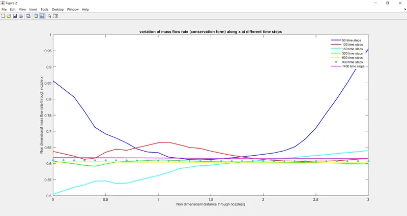
    figure(2)
    if j==50
        plot(x,cons_mass_flow,'b','linewidth',1.5);
        hold on 
    elseif j==100
        plot(x,cons_mass_flow,'r','linewidth',1.5)
        hold on 
    elseif j==150
        plot(x,cons_mass_flow,'c','linewidth',1.5)
        hold on 
    elseif j==300
        plot(x,cons_mass_flow,'g','linewidth',1.5)
        hold on 
    elseif j==600
        plot(x,cons_mass_flow,'y','linewidth',1.5)
        hold on 
    elseif j==900
        plot(x,cons_mass_flow,'*','linewidth',1.5)
        hold on 
    elseif j==1400
        plot(x,cons_mass_flow,'m','linewidth',1.5)
        hold on 
    
    
    end
end
xlabel('Non dimensioanl distance through nozzle(x)','fontsize',10)
ylabel('Non dimensional mass flow rate through nozzle x','fontsize',10);
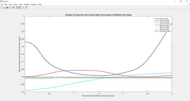
title('variation of mass flow rate (conservation form) along x at different time steps');
  legend({'50 time steps','100 time steps','150 time steps','300 time steps','600 time steps','900 time steps','1400 time steps'});
end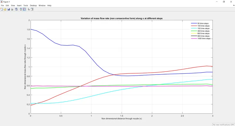

Grid Dependence test :

This test mainy to to determine all the primitive variable ratios at  different grid points mainly at n=31 and n=61 etc.

Primate variables and condition at nozzle

		Density ratio ρρo">ρ/ρo	Temperature ratio TTo">T/To	Pressure ratio PPo">P/Po	Mach number M">M
n=31	non conservative	0.6387	0.8365	0.5342	0.9994
n=61	non conservative	0.6377	0.8354	0.5327	0.9998
n=31	conservative	0.6642	0.8939	0.5937	0.9801
n=61	conservative	0.6424	0.8601	0.5525	1.0008

Exact solution

0.634

0.833

0.528

1.00

Simulation time data:

grid points		time for simulation
n=31	non conservative	3.1510
n=31	conservative	2.952
n=61	non conservative	3.2231
n=61	conservative	3.0038

CFL data effect  on  non coservative form for 31 grid points:

CFL number	Density ratio ρρo">ρ/ρo	Temperature ratio TTo">T/To	Pressure ratio PPo">P/Po	Mach number M">M
0.5	0.6387	0.8365	0.5342	0.9994
0.8	0.6393	0.8367	0.5349	0.9991
1.0	0.6397	0.8368	0.5353	0.9988
1.1	0.6399	0.8369	0.5355	0.9987
1.2	----------	-----------	-----------	--------

Exact solution

0.634

0.833

0.528

1.00

The solution blew at CFL value equal to 1.2

CFL data effect  on   coservative form for 31 grid points:

CFL number	Density ratio ρρo">ρ/ρo	Temperature ratio TTo">T/To	Pressure ratio PPo">P/Po	Mach number M">M
0.5	0.6642	0.8939	0.5937	0.9801
0.8	0.6642	0.8939	0.5937	0.9801
1.0	0.6642	0.8939	0.5937	0.9801
1.1	0.6642	0.8939	0.5937	0.9801
1.2	0.6642	0.8939	0.5937	0.9801

Exact solution

0.634

0.833

0.528

1.00

The CFL  value does not have any effect on conservative form primate variables ratio.

From the table it can be seen that as we increase the number of grid points we could say that  the value approaches very close to the analytical solution.But however the increase in number of grid points increases the simulation time required to run the program.

• The time taken for simulation in case of conservative form is lesser as comapred to non conservative form as shown in the simulation table data.
• In grid dependence test we observe that the accuracy in case of non consevative form is more as comapared to conservative form as it is very close to exact analytical solution.
• The conservative form provides more accuracy incase of mass flow rate whereas non conservative provide more accuracy in case of primitive variables .However in general we can say that non conservative form has higher accuracy than conservative form.
• No For the first table of cfl effects signifies about the effect on non conservative form.It is observed that as CFL value increases the density,pressure and Temperature ratio increases.But however mach number decreases.For  the cfl value 1.2 the sloution gets blown off . No wonder it is the threshold CFL value . 
• In the second table it represents data for conservative form the increase or decrease in cfl value doesnt effect the solution itself.