Simulation of a 1D Super-sonic nozzle flow simulation using Macormack Method
Objective:
1. To simulate a 1D Quasi subsonic-supersonic flow inside a convergent-divergent nozzle with 2nd order accuracy using MacCormack's Explicit Method.
2. To compare the numerical results obtained from both conservative form and non-conservative form with the analytical results and draw a line of superiority based on the comparison
3. Accomplish mesh independence test and CFL based adaptive time loop control to be programmed to assure the fidelity of the numerical results
Introduction & Problem Statement:
Here we have considered a steady, isentropic flow through a convergent-divergent nozzle as in Fig. 1. The flow at the inlet to the nozzle comes from a reservoir where the pressure and temperature are denoted by `p_0` and `T_0` respectively. The cross-sectional area of the reservoir is large (theoretically `A -> infty`) and hence the velocity is very small (`V-> infty`). This `p_0` and `T_0` are the stagnation values or total pressure and total temperature respectively. The flow expands isentropically to supersonic speeds at the nozzle exit where the exit pressure, temperature, velocity and match number are denoted by `p_e, T_e, V_e` and `M_e` respectively.
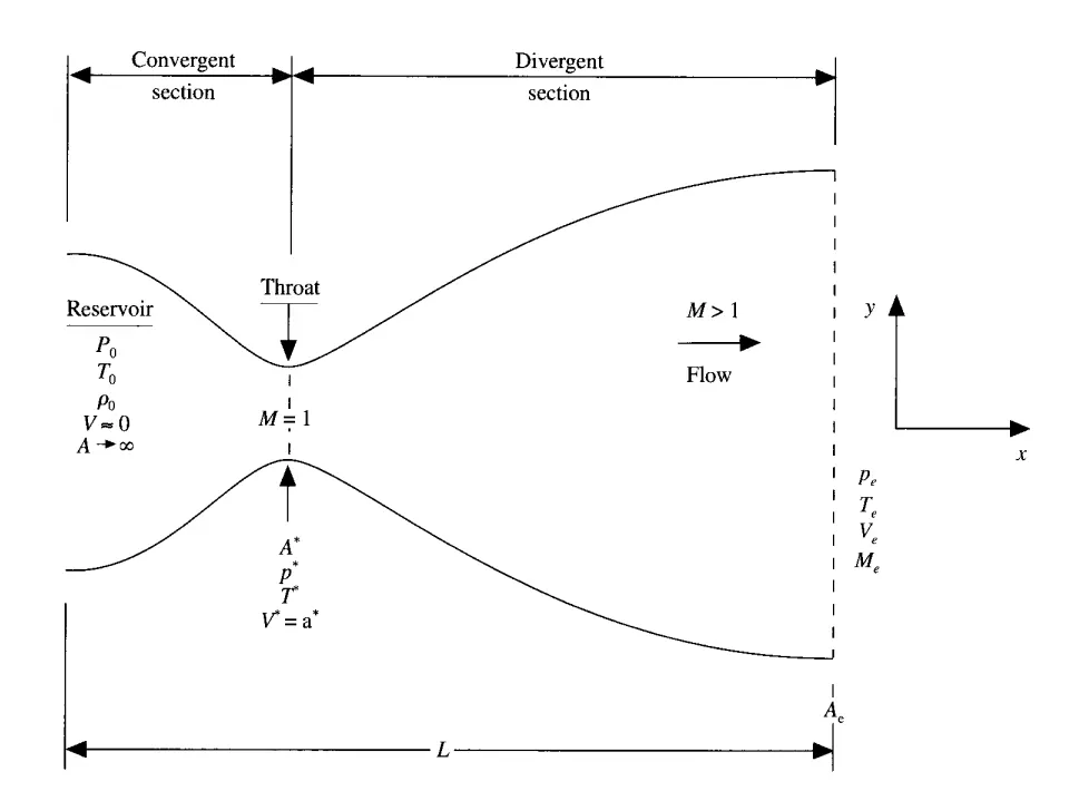
Figure: 1: Schematic diagram of subsonic-supersonic isentropic nozzle flow
The flow is locally subsonic in the convergent section of the nozzle, sonic at the throat (minimum area) and supersonic at the divergent section. The sonic flow (M = 1 ) at the throat means that the local velocity at this location is equal to the local speed of sound, V=V*=a*. Asterisk is used to denote sonic values. Similarly, the sonic values of pressure and temperature are p* and T* respectively. The area is also denoted by A* at the throat.
Nozzle Shape: `A =1+2.2(x-1.5)^2` `0<=x<=3`
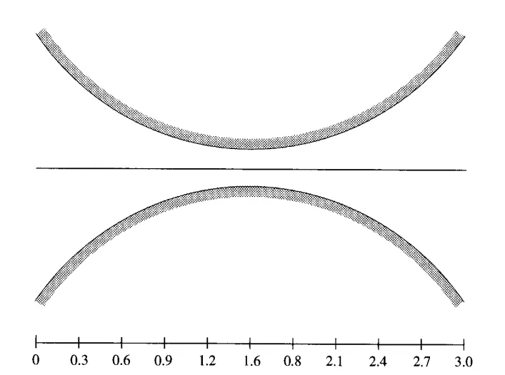
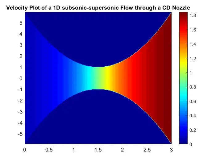
Figure: 2: Non-dimensional Distance along with the nozzle
Assumptions for Mathematical Modelling:
1. Here we have considered the flow is 1D quasi flow i.e the flow properties changes only in the x-direction though, in reality, the flow is 2D. This is twisting the real physics of the flow and we are basically, trying to consider an inviscid flow in this case.
2. We are considering the gas flowing through the Convergent-Divergent (CD) nozzle to be calorically perfect gas.
3. No Shock formation is taking place at the supersonic section of the nozzle.
Governing Equations:
Continuity: `rho_1V_1A_1 = rho_2A_2V_2`
Momentum: `p_1A_1 + rho_1V_1^2A_1 + int_(A_1)^(A_2) pdA = p_2A_2 + rho_2V_2^2A_2`
Energy: `h_1 + V_1^2/2 = h_2 + V_2^2/2`
But to continue further we need to convert this integral form to differential form which can be either in non-conservational form or conservation form. We will represent all the parameters in both the forms in non-dimensional form to get a better visualization of solution pattern.
1. Non-dimensionalized Non-conservative Form of Governing Equation:
Continuity: `(delp')/(delt') =rho'(delV')/(delx') - rho'V'(del(lnA'))/(delx')-V'(delp')/(delx')`
Momentum: `(delV')/(delt')=-V'(delV')/(delx') - 1/gamma((delT')/(delx')+(T')/(rho')(delrho')/(delx'))`
Energy: `(delT')/(delt')=-V'(delT')/(delx')-(gamma-1)T'[(delV')/(delx')+V'(del(lnA'))/(delx')]`
Intiial Conditions:
`rho=1.0-0.3146x`
`T=1.0-0.2314x`
`V=(0.1+1.09x)T^(1/2)`
Boundary Conditions:
Inlet:
`v(1 )= 2v(2) -v(3)`
Outlet:
`v(n) = 2v(n-1) -v(n-2)`
`rho(n)=2rho(n-1)-rho(n-2)`
`T(n) = 2T(n-1)-T(n-2)`
2. Non-dimensionalized Conservative Form of Governing Equation:
Continuity: `(delU_1)/(delt') = -(delF_1)/(delx')`
Momentum:`(delU_2)/(delt') = -(delF_2)/(delx') + J_2`
Energy:`(delU_3)/(delt') = -(delF_3)/(delx')`
Where U is the solutions vectors, F is the flux vectors and J is the source term
`U_1 = rho'A'`
`U_2=rho'A'V'`
`U_3=rho'((e')/(gamma-1) + (gamma)/2V'^2)A'`
`F_1=rho'A'V'`
`F_2= rho'A'V'^2 +1/gammap'A'`
`F_3=rho'((e')/(gamma-1)+gamma/2V'^2)V'A'+p'A'V'`
`J_2=1/gammap'(delA')/(delx')`
After solving these equations we can get back to our desired parameters by using the following equations:
`rho' = U_1/(A')`
`V' = U_2/U_1`
`T'=e'=(gamma-1) ((U_3)/(U_1)-gamma/2V'^2)`
`p'=rho'T'`
Initial Conditions:
`{:(rho'=1.0),(T'=1.0):} } -> 0<=x'<=0.5`
`{:(rho'=1.0-0.366(x'-0.5)),(T'=1.0-0.167(x'-0.5)):} } -> 0.5<=x'<=1.5`
`{:(rho'=0.634-0.3879(x'-1.5)),(T'=0.833-0.3507(x'-1.5)):} } -> 1.5<=x'<=3.5`
Boundary Conditions:
Inlet:
`U_1 = rho(1) A(1)`
`U_2(1) = 2U_2(2)-U_2(3)`
`U_3(1) = U_1(1)[(T(1))/(gamma-1) + gamma/2v(1)^2]`
Outlet:
`U_1(n) = 2U_1(n-1)-U_1(n-2)`
`U_2(n) = 2U_2(n-1) - U_2(n-2)`
`U_3(n) = 2U_3(n-1) - U_3(n-2)`
Lets now discuss the process
Maccormack Method
Steps that are included in MacCormack Method are as follows:
Step:1: Predictor Step: In this step, we set up the spatial derivatives as forward differences at time step t.
Step:2: Solution Update: In this step, we obtain the predicted values of the `rho, V and T` using the derivatives obtained from the predictor step.
Step:3: Corrector Step: Here we replace the spatial derivatives with rearward or backward difference method at time step `t + /_t`
Step:4: Calculating Average: Now we average the time derivatives obtained from both predictor and corrector method.
Step:5: Final Solution update:
At last, we calculate the final solution for the `rho, V and T`using the average values of the time derivates at `t + /_t`time step
CFL based Time-Step Calculation:
So one of the major challenges here is to figure out the value of time step. The governing equations are hyperbolic in nature with respect to time. So while considering the time step we need to keep in mind about the stability of the numerical solution. The stability constraint can be best defined by the following equation:
`t = C (/_x)/(a+V)`
Where,
t = time step
C = Courant Friedrichs Lowry (CFL) number
`/_x` = difference between one grid point to another
a = velocity of sound
V = velocity of the flow
This can also be stated as the non-dimensional form of the stability criteria as converting all the parameters here to non-dimensional form gives the same equation.
For linear hyperbolic equations stability is ensured for C <=1 for an explicit numerical solution. For which we set the time step in two ways. The first approach will lead us to an artificial time wrap and this will end up with various time step for each of the grid points. The second approach is the best way for unsteady problems which can lead us to a reliable solution. Here we will calculate the local time step for all the grid points and take the minimum of them.

This will be used as the time step. Such a way we can get a consistent time marching approach and thus creating a more physically sensible transient variation.
Code:
1. Main Code
close all
clear all
clc

%% INPUTS
n = 31;
L=3; %meter
x = linspace(0,L,n);
dx = x(2) - x(1);
nt = 1400;
CFL =0.5;
gamma=1.4;
%Nozzle Profile
A = 1 + 2.2*(x-1.5).^2;
%% Non Conservative part
[P,T,rho,v,M,m,P_t,T_t,rho_t,v_t,M_t,residuals,dt] = nonconservative_Test(n,x,dx,A,CFL,nt,gamma);
%% Conservative part
[Pc,Tc,rhoc,vc,Mc,mc,U1,U2,U3,P_tc,T_tc,rho_tc,v_tc,M_tc,residualsc,dtc] = conservative_Test(n,x,dx,A,CFL,nt,gamma);

%% plotting Non-Conservations Governing Equations

figure(1)
subplot(4,1,1)
plot(x,M,'LineWidth',1.3)
ylabel("Mach Number")
title("Qualitative aspects of quasi 1D nozzle flow: Non-Conservation Governing Equations")
subplot(4,1,2)
plot(x,P,'LineWidth',1.3)
ylabel("Pressure ratio")
subplot(4,1,3)
plot(x,rho,'LineWidth',1.3)
ylabel("Density ratio")
subplot(4,1,4)
plot(x,T,'LineWidth',1.3)
ylabel("Temperature ratio")
xlabel("x")

figure(2)
subplot(4,1,1)
plot(x,Mc,'LineWidth',1.3)
ylabel("Mach Number")
title("Qualitative aspects of quasi 1D nozzle flow: Conservation Governing Equations")
subplot(4,1,2)
plot(x,Pc,'LineWidth',1.3)
ylabel("Pressure ratio")
subplot(4,1,3)
plot(x,rhoc,'LineWidth',1.3)
ylabel("Density ratio")
subplot(4,1,4)
plot(x,Tc,'LineWidth',1.3)
ylabel("Temperature ratio")
xlabel("x")

figure(3)
Nt=1:1:nt;
subplot(4,1,1)
plot(Nt,M_t,Nt,M_tc,'LineWidth',1.3)
legend("Non-conservative","Conservative")
ylabel("Mach Number")
title("Flow Parameters with time steps at the throat")
subplot(4,1,2)
plot(Nt,P_t,Nt,P_tc,'LineWidth',1.3)
legend("Non-conservative","Conservative")
ylabel("Pressure ratio")
subplot(4,1,3)
legend('Non-conservative','Conservative')
plot(Nt,rho_t,Nt,rho_tc,'LineWidth',1.3)
ylabel("Density ratio")
subplot(4,1,4)
plot(Nt,T_t,Nt,T_tc,'LineWidth',1.3)
legend("Non-conservative","Conservative")
ylabel("Temperature ratio")
xlabel("Time Steps, nt")

figure(4)
for var=1:n
    actual_mass_flow_rate(var) = 0.579;
end
plot(x, m(nt,:),'o-',x,U2,'o-',x,actual_mass_flow_rate,'o-','LineWidth',1.3)
title("Mass Flow Rate vs x")
xlim([0 3])
legend('Non-Conservative Form','Conservative Form','Exact Mass Flow Rate')

figure(5)
plot(x,m(50,:),'o-',x,m(100,:),'o-',x,m(150,:),'o-',x,m(200,:),'o-',x,m(700,:),'o-','LineWidth',1.3)
legend("t=50Deltat","t=100Deltat","t=150Deltat","t=200Deltat","t=700Deltat")
xlabel("x")
ylabel("rhoAV/rho_0A_0V_0")
ylim([0 2.3])
title('Variation of Non-dimensional Mass Flow Rate Non-Conservative Form')
grid on

figure(6)
plot(x,mc(100,:),'o-',x,mc(150,:),'o-',x,mc(200,:),'o-',x,mc(700,:),'o-','LineWidth',1.3)
legend("t=50Deltat","t=100Deltat","t=150Deltat","t=200Deltat")
xlabel("x")
ylabel("rhoAV/rho_0A_0V_0")
%ylim([0 2.3])
title('Variation of Non-dimensional Mass Flow Rate Conservative Form')
grid on

%%Residuals
figure(7)
plot(Nt,residuals(:,1),'o-',Nt,residuals(:,2),'o-',Nt,residuals(:,3),'o-','LineWidth',1.2)
title("Residuals Non-Conservative Form")
xlim([0 nt])
ylim([0 max(max(residuals))])
xlabel("Time Step")
ylabel("Residuals")

figure(8)
plot(Nt, residualsc(:,1),'o-',Nt,residualsc(:,2),'o-',Nt,residualsc(:,3),'o-','LineWidth',1.2)
title("Residuals Conservative Form")
xlim([0 nt])
ylim([0 max(max(residualsc))])
xlabel("Time Step")
ylabel("Residuals")
2. user defined function: nonconservative_Test()
function [P,T,rho,v,M,m,P_t,T_t,rho_t,v_t,M_t,residuals,dt] = nonconservative_Test(n,x,dx,A,CFL,nt,gamma)
    %% Initial Profiles
    rho = 1-0.3146*x;
    T = 1-0.2314*x;
    v = (0.1 + 1.09*x).*T.^0.5;
    v_initial =v;
    throat=find(A ==1);
    residuals=zeros(nt,3);
    %% Time Steps
    dt = min(CFL *(dx./(T.^0.5 +v)));
    %% Non-Conversative
    %Time Loop
    for k = 1:nt

        rho_old=rho;
        v_old = v;
        T_old =T;

    %Space Loop
        for i = 2:n-1
            %Predictor terms
            %Forward Difference Method
            dvdx = (v(i+1) - v(i))/dx;
            drhodx = (rho(i+1) - rho(i))/dx;
            dTdx = (T(i+1) - T(i))/dx;
            dlogAdx = (log(A(i+1)) - log(A(i)))/dx;

            %Main N-S Eqns
            drhodt_p(i) = -rho(i)*dvdx - rho(i)*v(i)*dlogAdx - v(i)*drhodx;
            dvdt_p(i) = -v(i)*dvdx - (1/gamma)*[dTdx + (T(i)/rho(i))*drhodx];
            dTdt_p(i) = -v(i)*dTdx - [(gamma-1)*T(i)]*[dvdx + v(i)*dlogAdx];

            %Updated Values
            rho(i) = rho(i) + drhodt_p(i)*dt;
            v(i) = v(i) + dvdt_p(i)*dt;
            T(i) = T(i) + dTdt_p(i)*dt;
        end

        for i = 2: n-1
            %Corrector terms
            %Backward Difference Method
            dvdx = (v(i) - v(i-1))/dx;
            drhodx = (rho(i) - rho(i-1))/dx;
            dTdx = (T(i) - T(i-1))/dx;
            dlogAdx = (log(A(i)) - log(A(i-1)))/dx;

            %Main N-S Eqns
            drhodt_c(i) = -rho(i)*dvdx - rho(i)*v(i)*dlogAdx - v(i)*drhodx;
            dvdt_c(i) = -v(i)*dvdx - (1/gamma)*[dTdx + (T(i)/rho(i))*drhodx];
            dTdt_c(i) = -v(i)*dTdx - [(gamma-1)*T(i)]*[dvdx + v(i)*dlogAdx];
        end

           drhodt = 0.5*(drhodt_p + drhodt_c);
           dvdt = 0.5*(dvdt_p + dvdt_c);
           dTdt = 0.5*(dTdt_p + dTdt_c);
        %% residuals
        residuals(k,1) = max(abs(drhodt));
        residuals(k,2) = max(abs(dvdt));
        residuals(k,3) = max(abs(dTdt));
        for i =2:n-1
           rho(i) = rho_old(i) + drhodt(i)*dt;
           v(i) = v_old(i) + dvdt(i)*dt;
           T(i) = T_old(i) + dTdt(i)*dt;
        end

        %Applying BC
        %inlet
        v(1) = 2*v(2)-v(3);

        %Outlet
        v(n) = 2*v(n-1) - v(n-2);
        rho(n) = 2*rho(n-1) - rho(n-2);
        T(n) = 2*T(n-1) -T(n-2);
    %% Post calculations:

    P = rho.*T;
    m(k,:)= rho.*A.*v ; %mass flow rate
    av=T.^0.5; %local velocity of sound
    M=v./av;

    %At throat
    P_t(k) = P(throat);
    T_t(k) = T(throat);
    rho_t(k) = rho(throat);
    v_t(k) = v(throat);
    M_t(k) =M(throat);


    end
end
3. User-Defined Function: conservative_Test()
function [P,T,rho,v,M,m,U1,U2,U3,P_t,T_t,rho_t,v_t,M_t,residuals,dt] = conservative_Test(n,x,dx,a,CFL,nt,gamma)
%% Area (a)
throat = find(a==1);
%% Initial Profiles
for i = 1:n
    if x(i) >= 0 && x(i) < 0.5
        rho(i) = 1.0;
          T(i) = 1.0;
    elseif x(i) >= 0.5 && x(i) <1.5
        rho(i) = 1.0 - 0.366*(x(i)-0.5);
          T(i) = 1.0 - 0.167*(x(i)-0.5);
    elseif x(i) >= 1.5 && x(i) <= 3.5
        rho(i) = 0.634 - 0.3879*(x(i)-1.5);
          T(i) = 0.833 - 0.3507*(x(i)-1.5);
    end
end
v = 0.59./(rho.*a);
residuals=zeros(nt,3);
%% Tranferred Profile
e = T;  %nondimensional energy e~>e'=e/eo = Cv*T/Cv*To =T/To=T'~>t'~>t
U1 = rho.*a;
U2 = rho.*a.*v;
U3 = rho.*[(e./(gamma-1)) + (gamma/2).*v.^2].*a;
%% Time Steps
%nt = 1400;
%CFL =0.5;
time(1) =0;
%% Conversative Form Loop
    %% Time Loop
    for s = 1:nt
        %Calculating dt
        dt = min(CFL *(dx./(T.^0.5 +v)));
        %Storing old values
        U1_old = U1;
        U2_old = U2;
        U3_old = U3;
    %% Space Loop
    %%%%%%%%%Updating Flux Terms %%% This is the wrong part
            F1 = U2;
            F2   = [[U2.^2./U1] + [(gamma-1)/gamma]*[U3-((gamma/2)*(U2.^2./U1))]];
            F3   = [gamma*(U2.*U3./U1) - (gamma*(gamma-1)/2)*(U2.^3./U1.^2)];
            for j = 2 : n-1
                dadx = [a(j+1) - a(j)] /dx;
                J2(j)   = rho(j)*T(j)*dadx/gamma;
            end
    %% Predictor Loop
        for i = 2:n-1
    %%%%%%%%Forward Difference Method
            dF1dx   = [F1(i+1) - F1(i)] / dx;
            dF2dx   = [F2(i+1) - F2(i)] / dx;
            dF3dx   = [F3(i+1) - F3(i)] / dx;
    %%%%%%%%N-S Eqns
            %Continuity Equation
            dU1dt_p(i) = - dF1dx;
            %Momentum Equation
            dU2dt_p(i) = - dF2dx + J2(i);
            %Energy Equation
            dU3dt_p(i) = - dF3dx;
            drhodt_p(i) = [rho(i+1) - rho(i)]/dx;
            dTdt_p(i) = [T(i+1) - T(i)]/dx;
    %%%%%%%%Updated Values
            U1(i) = U1(i) + dU1dt_p(i)*dt;
            U2(i) = U2(i) + dU2dt_p(i)*dt;
            U3(i) = U3(i) + dU3dt_p(i)*dt;
        end

        rho = U1./a;
        v = U2./U1;
        T = (gamma-1)*[(U3./U1)-((gamma/2)*v.^2)];
    %%%%%%%%%Updating Flux Terms
            F1 = U2;
            F2   = [[U2.^2./U1] + [(gamma-1)/gamma]*[U3-((gamma/2)*(U2.^2./U1))]];
            F3   = [gamma*(U2.*U3./U1) - (gamma*(gamma-1)/2)*(U2.^3./U1.^2)];
            for j = 2 : n-1
                dadx = [a(j) - a(j-1)] /dx;
                J2(j)   = rho(j)*T(j)*dadx/gamma;
            end
    %% Corrector Loop
        for z = 2: n-1
    %%%%%%%%%Backward Difference Method
            dF1dx   = [F1(z) - F1(z-1)] / dx;
            dF2dx   = [F2(z) - F2(z-1)] / dx;
            dF3dx   = [F3(z) - F3(z-1)] / dx;
    %%%%%%%%N-S Eqns
            %COntinuity Equation
            dU1dt_c(z) = - dF1dx;
            %Momentum Equation
            dU2dt_c(z) = - dF2dx + J2(z);
            %Energy Equation
            dU3dt_c(z) = - dF3dx;
        end
    %% Calculating Final U terms
           dU1dt = 0.5*(dU1dt_p + dU1dt_c);
           dU2dt = 0.5*(dU2dt_p + dU2dt_c);
           dU3dt = 0.5*(dU3dt_p + dU3dt_c);
        %% residuals
            residuals(s,1) = max(abs(dU1dt));
            residuals(s,2) = max(abs(dU2dt));
            residuals(s,3) = max(abs(dU3dt));
        %% continue Calculating the Final U
        for d =2:n-1
           U1(d) = U1_old(d) + dU1dt(d)*dt;
           U2(d) = U2_old(d) + dU2dt(d)*dt;
           U3(d) = U3_old(d) + dU3dt(d)*dt;
        end
        %% Applying BC
        %% Inlet
        U1(1) = rho(1)*a(1); %% Not necessary to assign again
        U2(1) = 2*U2(2)-U2(3);
        U3(1) = U1(1)*[T(1)/(gamma-1) + (gamma/2)*v(1)^2];  %% Not necessary to assign again
        %% Outlet
        U1(n) = 2*U1(n-1) - U1(n-2);
        U2(n) = 2*U2(n-1) - U2(n-2);
        U3(n) = 2*U3(n-1) - U3(n-2);
    %% Retrieving the original parameter from U terms
        rho = U1./a; % rho = u1/a' a' =a x a*
        v = U2./U1;
        T = (gamma-1)*[(U3./U1)-((gamma/2)*v.^2)];
        e=T;
        P = rho.*T;
        m(s,1:n)= rho.*a.*v; %U2
        M = v./(T.^0.5);
        %At throat
        P_t(s)=P(throat);
        T_t(s)=T(throat);
        v_t(s)=v(throat);
        rho_t(s)=rho(throat);
        M_t(s)=M(throat);
    end
end
Algorithm:
1. First we have entered the inputs like the number of grid points, CFL number, nozzle profile, total number of time steps for which the simulation will run to reach the final solution.
2. After that we call the functions converative() and nonconsercative() to get the results
3. After obtained the primitive parameters we plotted the necessary graphs to get to the conclusion.
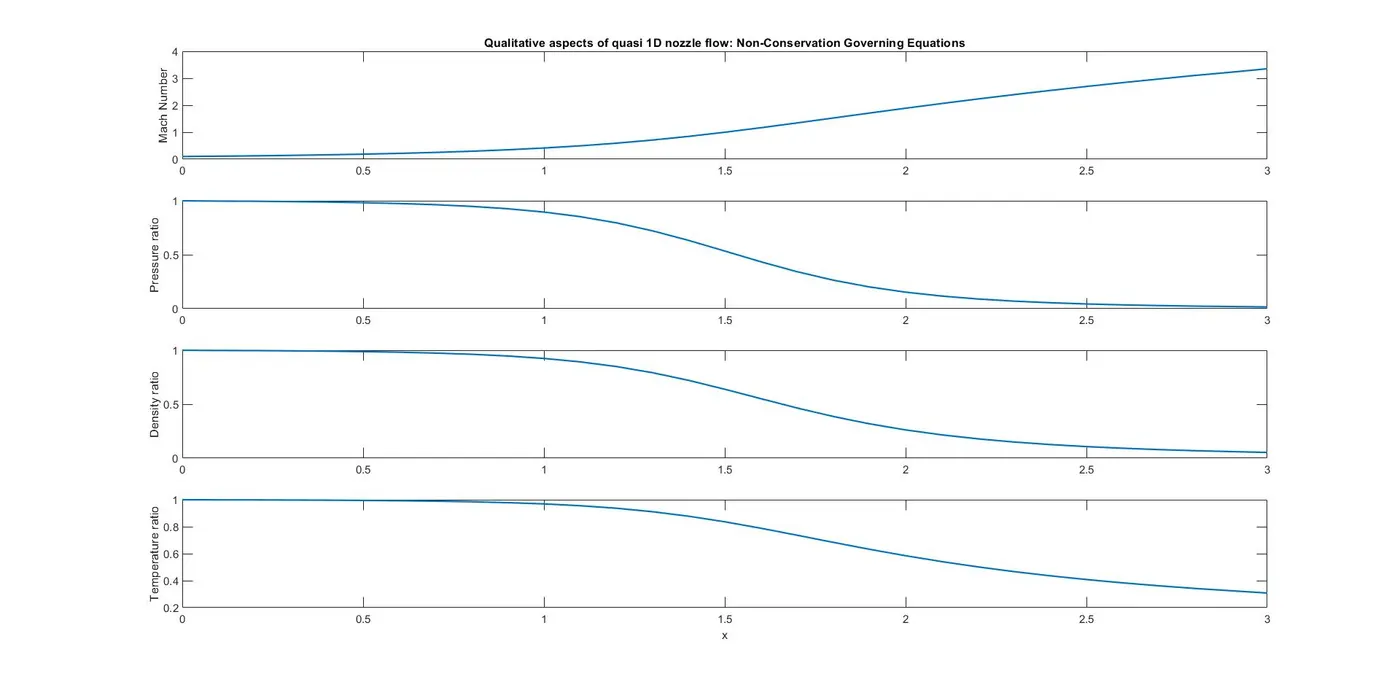
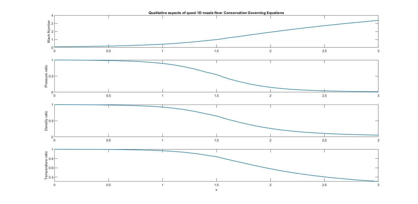
Graphs:
Mesh Independence Test:
In Summarized Form:
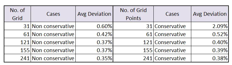
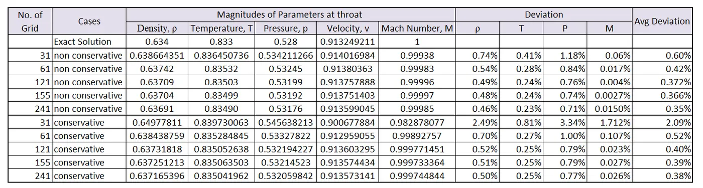
So we can see that the no significant changes in the values are obtained even after making the mesh fine by doubling the number of grid points from 31 to 61 points. So we can get reliable results with 31 grid points.
Result and Discussion:
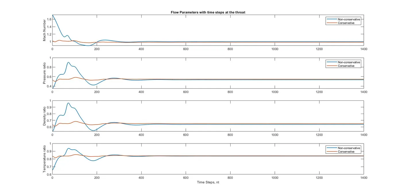
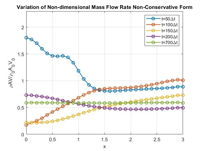
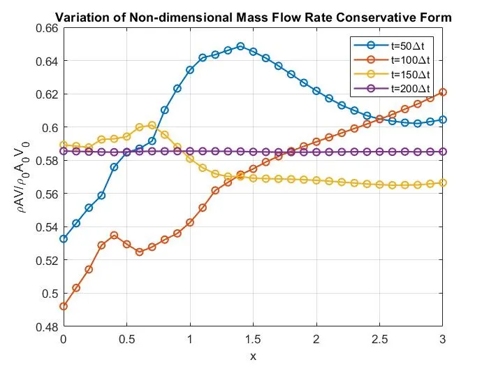
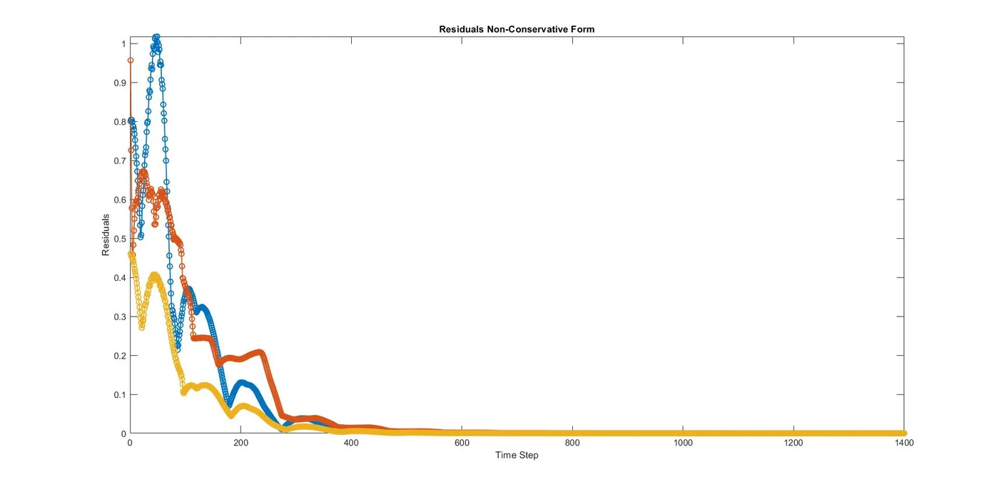
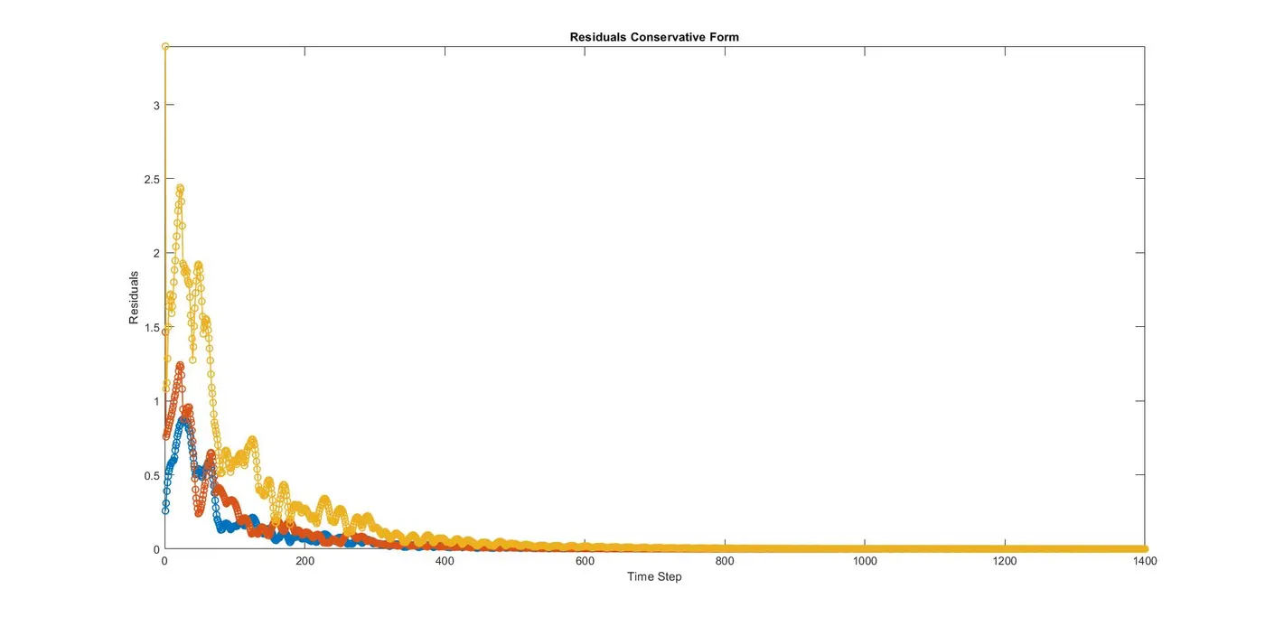
1. Non-conservative is faster than conservative form and the final solution is obtained only in 900-time steps whereas for conservative form it takes 1400 time steps to get the final solutions. This is applicable for 31 grid points only. For finer grid points we need more number of time steps to reach final solution.
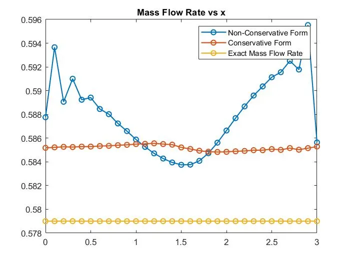
2. For the same number of grid points, non-conservative forms better approximation than the conservative form as compared to the exact solution obtained from experiments. But Conservative form provides a better approximation for the mass flow rate and this is because of the truncation error. See in the conservation form we are directly getting the mass flow rate as one of the solution of the governing equation that is `U_2` but in case of non-conservative form, we need to multiply the primitive parameters to get the mass flow rate and thus leading to truncation error.
Conclusion: So it is hard to conclude which one is better in terms of accuracy and draw a clear line of supremacy but in terms of getting faster and accurate results non-conservative form is obviously a better approach.
Reference: John D. Anderson, Jr (1992). Disrupters: Computational Fluid Dynamics: The Basics with Application. the mold. Springer Science & Business Media