Solving Steady and Unsteady heat conduction equation of a 2D plate surrounded by constant temperature by Finite Difference Method

Objective:

To solve a heat conduction equation of a 2D plate surrounded by constant temperature by Finite Difference Method. Here we will consider both the steady-state and transient cases and compare by which iterative method results with better accuracy with less number of iteration can be obtained. Also, we will try to understand the effect of CFL number in case of transient case.

Assumption:

1. Absolute error criteria is 1e-4

2. Considered equal number of grid points or nodes along the X-axis and Y-axis

3. No internal heat generation

4. Boundary Conditions are as follows

Top Boundary = 600 K

Bottom Boundary = 900 K

Left Boundary = 400 K

Right Boundary = 800 K

Governing Equation:

`(del^2T)/(delx^2) + (del^2T)/(dely^2) + (del^2T)/(delz^2) + dotq /k= (rhoc_p)/(k) (delT)/(delt)`

Here,

`dot q` = Rate of Heat Generation

`k`= Thermal Conductivity

`rho`= Density

`c_p`= Specific heat capacity at constant pressure

`rhoc_p`=volumetric heat capacity

Considering 2D case and no heat generation constant Pressure

`=> (del^2T)/(delx^2) + (del^2T)/(dely^2) = 1/alpha(delT)/(delt)`

`=> (delT)/(delt) = alpha [(del^2T)/(delx^2) + (del^2T)/(dely^2)]`

Numerical Discretization:

1. Steady Case

In case of steady-state the time derivative term of temperature becomes zero. So the governing equation becomes:

`(del^2T)/(delx^2) + (del^2T)/(dely^2) = 0`

Now Discretizing each of the terms bu finite difference method we get,

`(del^2T)/(delx^2) = [T_(i,j+1)^(n) + 2T_(i,j)^(n) +T_(i,j-1)^(n) ]/ (/_x)^2`

`(del^2T)/(dely^2) = [T_(i+1,j)^(n) + 2T_(i,j)^(n) +T_(i-1,j)^(n) ]/ (/_y)^2`

`:.` After Calculation

`T_(i,j) = [T_(i+1,j) + T_(i-1,j) +T_(i,j+1) + T_(i,j-1)]/4`

This simultaneous set of equation can be solved by the following iterative methods:

• Jacobi: `T_p = T_(old_T) +T_(old_B) +T_(old_L) +T_(old_R)`
• Gauss-Seidel: `T_p = T_T + T_(old_B) + T_L + T_(old_R)`
• Successive Order Reduction: `T_(P_(SOR)) = (1- omega)T_(P_(old)) + omegaT_(P_(GS))`

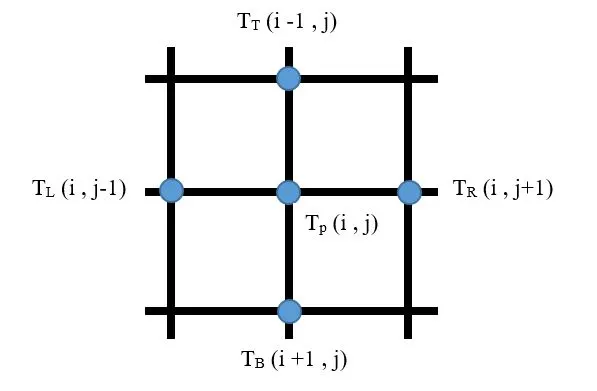
Here the subscript old refers to the values in the previous iteration and the subscripts T, B, R and L refers to Top, Botton, Right and Left respectively. The following graphics illustrate the notation that has used here in stating the equations.

2. Transient Case

In the case of the transient case the time derivative term of temperature is considered. So the governing equation becomes:

`alpha((del^2T)/(delx^2) + (del^2T)/(dely^2)) = (delT)/(delt)`

Here,

`alpha = k/(rhoc_p)` = 1.4 `m^2/s`(Considered arbitrarily)

Now Discretizing each of the terms by finite difference method we get,

`(delT)/(delt) = (T_l^(n+1) - T_l^n )/(/_t)`

Now we can get two cases, Explicit and Implicit based on the discretization of the remaining two terms.

Considering previous time steps will give rise to explicit terms and considering same time steps will give rise to the implicit case

Explicit Case:

`(del^2T)/(delx^2) = [T_(i,j+1)^(n) + 2T_(i,j)^(n) +T_(i,j-1)^(n) ]/ (/_x)^2`

`(del^2T)/(dely^2) = [T_(i+1,j)^(n) + 2T_(i,j)^(n) +T_(i-1,j)^(n) ]/ (/_y)^2`

`:.` After Calculation considering `/_x = /_ y` and k1 = k2

`T_(P)= T_(P_(old))[1-4k] + k(T_(T_(old)) +T_(B_(old)) +T_(L_(old))+ T_(R_(old)))`

Implicit Case:

`(del^2T)/(delx^2) = [T_(i,j+1)^(n+1) + 2T_(i,j)^(n+1) +T_(i,j-1)^(n+1) ]/ (/_x)^2`

`(del^2T)/(dely^2) = [T_(i+1,j)^(n+1) + 2T_(i,j)^(n+1) +T_(i-1,j)^(n+1) ]/ (/_y)^2`

`:.` After Calculation considering `/_x = /_ y` and k1 = k2

`T_(P)= [T_(P_(prev)) + k(T_R+T_B+T_T+T_B)]/[1+4k]`

Now just like the steady state equations this set of implicit case can be solved by the following iterative methods.
Here `T_(P_(prev))` = value of `T_P`in the previous time step

• Jacobi
• Gauss-Seidel
• Successive Order Reduction

Code:

1. Main Code:

%%%%%%%%%%%%%%%%%%%%%%%%%%%%%%%%%%%%%%%%%%%%%%%%%%%%%
%%%%%%%%%%%%%%%%%%%%%%%%%%%%%%%%%%%%%%%%%%%%%%%%%%%%%
%% Code History
% Author: Arghya Kamol Roy
% Date: 26 April 2020
%Problem: 2D Heat Conduction Problem 1
%%%%%%%%%%%%%%%%%%%%%%%%%%%%%%%%%%%%%%%%%%%%%%%%%%%%%
%% %%%%%%%%%%%%%%%%%%%%%%%%%%%%%%%%%%%%%%%%%%%%%%%%%%%

clear all
close all
clc

%% Step 1: Inputs
L=1;
nx=11;
x=linspace(0,L,nx);
dx=x(2)-x(1);

W=1;
ny=nx;
y=linspace(0,W,ny);
dy=y(2)-y(1);

prompt = 'type= ' %Transient Case =1 and Steady State =2
type = input(prompt);

if type == 1 
    prompt = 'CFL= '
    CFL = input(prompt); %Fails for Explicit if CFL >0.5 
                         %CFL=CFLx+CFLy = alpha*dt/dx^2 + alpha*dt/dy^2 = 2*alpha*dt/dx^2
else CFL =0
end
alpha = 1.4; 

%% Step 2: Finding dt & nt
dt=CFL*dx^2/(2*alpha);
time = .03*60; % mins
nt = time/dt;

%% Step 3: Error Limit Inputs
error=9e9;
tol=1e-4;

%% Step 4: Boundary COnditions
T=300*ones(nx,ny);
T(:,1) = 400; %kelvin
T(:,end) = 800;
T(1,:) = 600; %top
T(end,:) = 900;%bottom
T(1,1) = (400+600)/2;
T(end,end) = (800+900)/2;
T(end,1) = (400+900)/2;
T(1,end) = (600+800)/2;

Told = T;
Tprev=T;

k1=(alpha*dt/(dx^2));
k2=(alpha*dt/(dy^2));



%%%%%%%%%%%%%%Transient & Steady State%%%%%%%%%%%%
%% Step 5: Calling Solver
if type == 1 %transient case
    linear_eqn_solver_explicit(T,Told,nx,ny,nt,x,y,dx,dy,dt,k1,k2); % Transient Explicit
    linear_eqn_solver_jacobi(T,Told,Tprev,nx,ny,nt,x,y,dx,dy,dt,k1,k2,tol,error,11);
    linear_eqn_solver_GS(T,Told,Tprev,nx,ny,nt,x,y,dx,dy,dt,k1,k2,tol,error,12);
    optimize_SOR(T,Told,Tprev,nx,ny,nt,x,y,dx,dy,dt,k1,k2,tol,error,13)
elseif type == 2  %Steady state case
    linear_eqn_solver_jacobi(T,Told,Tprev,nx,ny,nt,x,y,dx,dy,dt,k1,k2,tol,error,21);
    linear_eqn_solver_GS(T,Told,Tprev,nx,ny,nt,x,y,dx,dy,dt,k1,k2,tol,error,22);
    optimize_SOR(T,Told,Tprev,nx,ny,nt,x,y,dx,dy,dt,k1,k2,tol,error,23)
end

User-Defined Functions:

1. linear_eqn_solver_jacobi

function linear_eqn_solver_jacobi(T,Told,Tprev,nx,ny,nt,x,y,dx,dy,dt,k1,k2,tol,error,type)
%%%%%%%Transient Implicit (Jacobi) %%%%%%%%%%%
    if type == 11
        tic;
        iteration_no =1;
        for k=1:nt %time loop 
           error = 9e9;
               while(error > tol) %convergence loop 
                   for i=2:nx-1 %space loop 
                       for j=2:ny-1   
                           term1 = (1+(2*k1)+(2*k2))^-1;
                           V = Told(i-1,j) + Told(i+1,j);
                           H =  Told(i,j-1) + Told(i,j+1);
                           T(i,j) = (Tprev(i,j)*term1) + (k1*term1*H) + (k2*term1*V);  
                       end
                   end %end of space loop 
                   error = max(max(abs(Told-T)));
                   Told=T;
                   iteration_no = iteration_no + 1;
               end %end of convergence loop 
               Tprev=T;
        end %end of time loop 
        time =toc;
        %PLotting
        f1=figure(1)
        contourf(x,fliplr(y),T,'--','ShowText','on')
        colorbar
        colormap('jet')
        text =sprintf("2D Transient Heat Conduction-Implicit-JacobinNo. of iterations %fnTime of simulation %f Sec",iteration_no,time)
        title(text)

%%%%%%%Steady State (Jacobi) %%%%%%%%%%%
    elseif type == 21  
        iteration_no =1;
        tic;
        while(error > tol) %convergence loop 
                   for i=2:nx-1 %space loop 
                       for j=2:ny-1   
                           term1 = Told(i,j-1) + Told(i,j+1);
                           term2 = Told(i-1,j) + Told(i+1,j);
                           T(i,j) = (1/4)*(term1 + term2);  
                       end
                   end %end of space loop 
                   error = max(max(abs(Told-T)));
                   Told=T;
                   iteration_no = iteration_no + 1;
         end %end of convergence loop 
    time =toc;
    %PLotting
    f1=figure(1)
    contourf(x,fliplr(y),T,'--','ShowText','on')
    colorbar
    colormap('jet')
    text =sprintf("2D Steady State Heat Conduction-JacobinNo. of iterations %fnTime of simulation %f Sec",iteration_no,time)
    title(text)
    end
end

2. linear_eqn_solver_GS

function linear_eqn_solver_GS(T,Told,Tprev,nx,ny,nt,x,y,dx,dy,dt,k1,k2,tol,error,type)
%%%%%%%Transient Implicit (Gauss Seidal) %%%%%%%%%%%
   if type == 12 
    iteration_no =1;
    tic;
    for k=1:nt %Time Loop
        error =9e9;
           while(error > tol) %Convergence Loop
               for i=2:nx-1 %Space Loop
                   for j=2:ny-1
                       term1 = (1+(2*k1)+(2*k2))^-1;
                       V = T(i-1,j) + Told(i+1,j);
                       H =  T(i,j-1) + Told(i,j+1);
                       T(i,j) = (Tprev(i,j)*term1) + (k1*term1*H) + (k2*term1*V);  
                   end
               end %Space loop  end
                 error = max(max(abs(Told-T)));
                 Told=T;
                 iteration_no = iteration_no + 1;
           end %Convergence loop end
           Tprev= T;
    end %Time loop end
    time=toc;
    %PLotting
    f2=figure(2)
    contourf(x,fliplr(y),T,'--','ShowText','on')
    colorbar
    colormap('jet')
    text =sprintf("2D Transient Heat Conduction-Implicit-GSnNo. of iterations %fnTime of simulation %f Sec",iteration_no,time)
    title(text)
    
%%%%%%%Steady State Gauss Seidal %%%%%%%%%%%   
   elseif type == 22  
        iteration_no =1;
        %error = 9e9;
        tic;
        while(error > tol) %convergence loop 
                   for i=2:nx-1 %space loop 
                       for j=2:ny-1   
                           term1 = T(i,j-1) + Told(i,j+1);
                           term2 = T(i-1,j) + Told(i+1,j);
                           T(i,j) = (1/4)*(term1 + term2);  
                       end
                   end %end of space loop 
                   error = max(max(abs(Told-T)));
                   Told=T;
                   iteration_no = iteration_no + 1;
         end %end of convergence loop 
    time =toc;
    %PLotting
    f2=figure(2)
    contourf(x,fliplr(y),T,'--','ShowText','on')
    colorbar
    colormap('jet')
    text =sprintf("2D Steady State Heat Conduction-GSnNo. of iterations %fnTime of simulation %f Sec",iteration_no,time)
    title(text)
   end
end 

3. linear_eqn_solver_SOR

function [iteration_no T time] = linear_eqn_solver_SOR(T,Told,Tprev,nx,ny,nt,x,y,dx,dy,dt,k1,k2,tol,error,type,w)
%%%%%%%Transient Implicit (SOR) %%%%%%%%%%%
    if type == 13
    iteration_no =1;
    tic;
    for k= 1:nt %time loop 
       error =9e9;
       while(error > tol) %convergence loop 
           for i=2:nx-1 %space loop
               for j=2:ny-1
                   term1 = (1+(2*k1)+(2*k2))^-1;
                   V =  T(i-1,j) + Told(i+1,j); %Ttop(updated)  + Tbottom
                   H =  T(i,j-1) + Told(i,j+1); %Tleft(updated) + Tright
                   T_GS(i,j) = (Tprev(i,j)*term1) + (k1*term1*H) + (k2*term1*V);
                   T(i,j) = ((1-w)*Told(i,j)) + (w*T_GS(i,j)); 
               end
           end %end of space loop 
             error = max(max(abs(Told-T)));
             Told=T;
             iteration_no = iteration_no + 1;
       end % end of convergence loop 
        Tprev= T;
    end %end of time loop
    time=toc;
    
%%%%%%%Steady State SOR %%%%%%%%%%%    
    elseif type == 23  
        iteration_no =1;
        %error = 9e9;
        tic;
        while(error > tol) %convergence loop 
                   for i=2:nx-1 %space loop 
                       for j=2:ny-1   
                           term1 = T(i,j-1) + Told(i,j+1);
                           term2 = T(i-1,j) + Told(i+1,j);
                           T_GS(i,j) = (1/4)*(term1 + term2);
                           T(i,j) = ((1-w)*Told(i,j)) + (w*T_GS(i,j)); 
                       end
                   end %end of space loop 
                   error = max(max(abs(Told-T)));
                   Told=T;
                   iteration_no = iteration_no + 1;
         end %end of convergence loop 
    time=toc;

    end
end

4. optimize_SOR

function optimize_SOR(T,Told,Tprev,nx,ny,nt,x,y,dx,dy,dt,k1,k2,tol,error,type)

    w=0.1; 
    n=w:0.1:1.9;
    itr = zeros(length(n));
    T_out = zeros((nx*length(n)),ny);
    Time =zeros(length(n));
    l=1;
    for m=1:length(n)
        [iteration_no T time] = linear_eqn_solver_SOR(T,Told,Tprev,nx,ny,nt,x,y,dx,dy,dt,k1,k2,tol,error,type,w); %type = 13 Implicit SOR or 23 SS SOR
        pause(0.01)
        w=w+0.1;
        itr(m) = iteration_no;
        T_out(0+l:(nx-1)+l,:) = T;
        l=l+nx;
        Time(m) = time;
        
        Tout=T;
        T=Tprev;
    end
    
    %plotting optimized graph
    
    [Min ,index] = min(itr);
    
    f3=figure(3)
    contourf(x,fliplr(y),T_out((nx*max(index))+1:(nx*max(index))+nx,:),'--','ShowText','on')

    colorbar
    colormap('jet')
    if type == 13
        text1 =sprintf("Optimized 2D Transient Heat Conduction-Implicit-SORnNo. of iterations %fnTime of simulation %f Secnw = %f", itr(max(index)),Time(max(index)),n(max(index)))
        title(text1)
    elseif type == 23
        text1 =sprintf("Optimized 2D Steady State Heat Conduction-SORnNo. of iterations %fnTime of simulation %f Secnw = %f", itr(max(index)),Time(max(index)),n(max(index)))
        title(text1)
    end
end

5. linear_eqn_solver_explicit

function linear_eqn_solver_explicit(T,Told,nx,ny,nt,x,y,dx,dy,dt,k1,k2)
%%%%%%%Transient Explicit%% %%%%%%%%%%% 
    iteration_no =1;
    tic;
    for k=1:nt %Time loop 
       for i=2:nx-1 %space loop 
           for j=2:ny-1
               term1 = (1- (2*k1)-(2*k2));
               H = Told(i+1,j) + Told(i-1,j);
               V =  Told(i,j+1) + Told(i,j-1);
               T(i,j) = (Told(i,j)*term1) + (k1*H) + (k2*V);  
           end
       end %end of space loop 
               error = max(max(abs(Told-T)));
               Told=T;
               iteration_no = iteration_no + 1;
    end %end of Time loop 
    time=toc;
    %PLotting
    f4=figure(4)
    contourf(x,fliplr(y),T,'--','ShowText','on')
    colorbar
    colormap('jet')
    text =sprintf("2D Transient Heat Conduction-Explicit-nNo. of iterations %fnTime of simulation %f Sec",iteration_no,time)
    title(text)
end

Algorithm:

1. Firstly we have defined the size of the 2D rectangle onto which we want to calculate the temperature contour. Then divided the geometry into equal grids points or node of equal length and width. After that, we have calculated the node sizes, dx and dy which are equal in magnitude that is dx =dy.

Then we accept the type of simulation we want to run that is whether a steady-state or transient case. Pressing "1" signifies transient case for which we take in another user input for CFL number and pressing "2" means steady-state.

2. From CFL number time step dt is automatically calculated. Here the total simulation time is set to 0.03 minute and from dt and total time we calculate the total number of time steps, nt.

3. In step 3 we define the boundary conditions which are as follows:

Top Boundary = 600 K

Bottom Boundary = 900 K

Left Boundary = 400 K

Right Boundary = 800 K

4. Then as per the type of simulation, the calculations are being done by the 5 user-defined functions namely, linear_eqn_solver_explicit(), linear_eqn_solver_jacobi(), linear_eqn_solver_GS(),linear_eqn_solver_SOR() and optimize_SOR() and prints the graphs along with the iteration number and simulation time.

5. Among this functions for the first 3 linear_eqn_solver_jacobi(), linear_eqn_solver_GS(),optimize_SOR() solves the steady state cases and transient cases are solved by the above mentioned 3 solvers and linear_eqn_solver_explicit(). The user defined function linear_eqn_solver_SOR() is called within optimize_SOR() all the time.

The main difference between these solvers are that they discretized equations are solved by different iteratives methods like jacobi, gauss-seidal or Successive Over Relaxation methods.

The main objective of optimize_SOR() function is the find the value of omega for which the number of iteration obtained using SOR method becomes the lowest.

Output:

1. Steady-State Analysis:

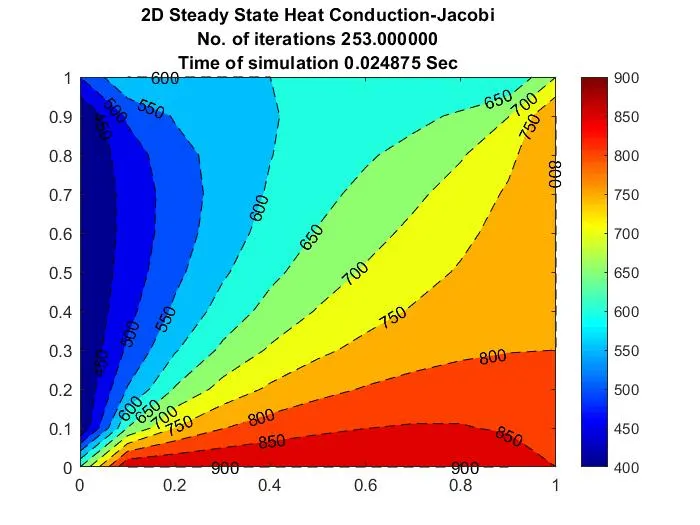
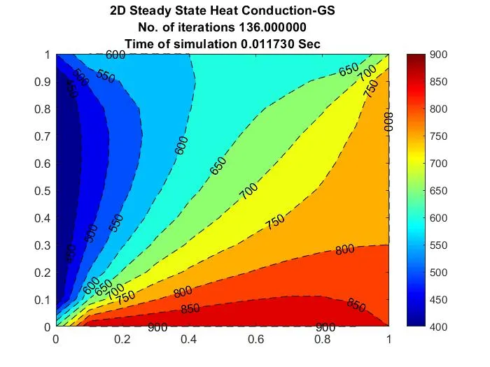
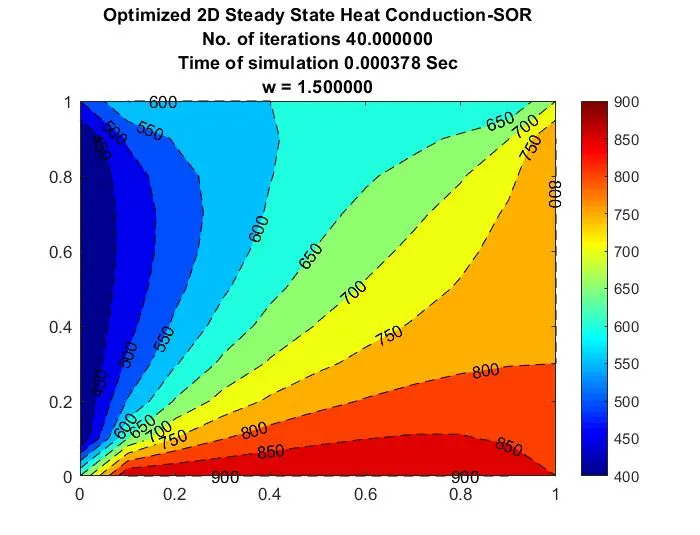
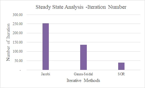
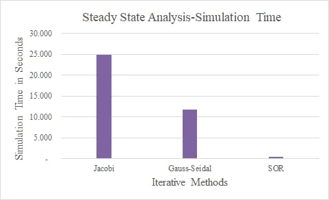
From the graphs, we get the following analytics

2. Transient Analysis:

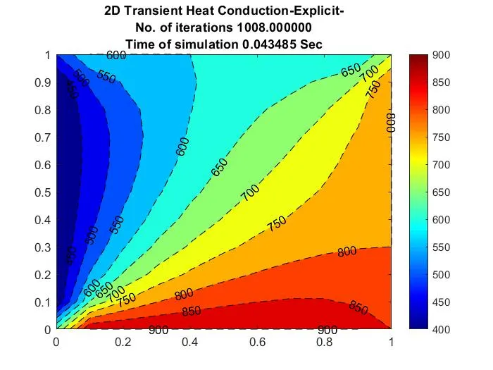
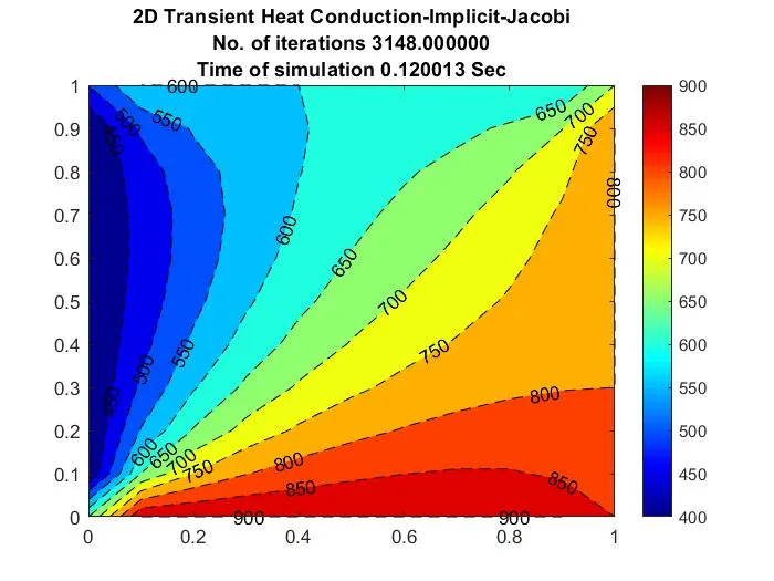
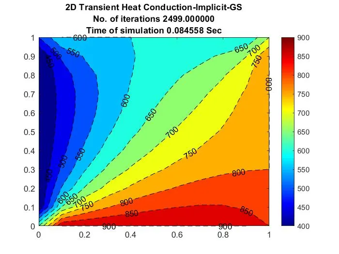
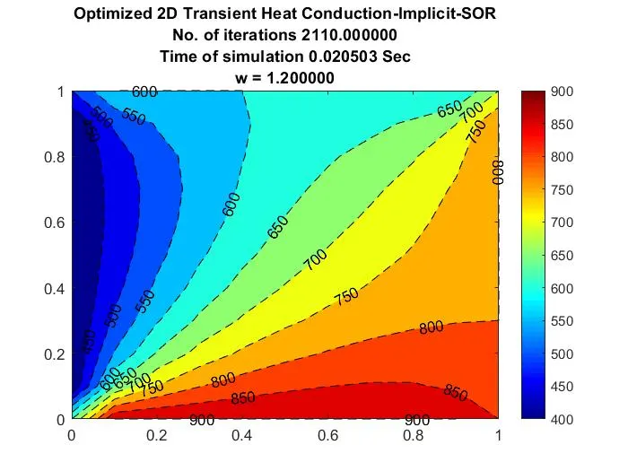
From the graphs, we get the following analytics

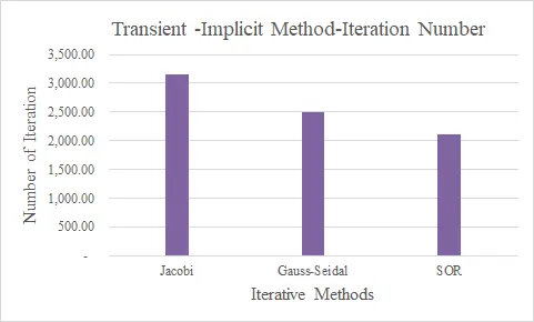
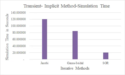
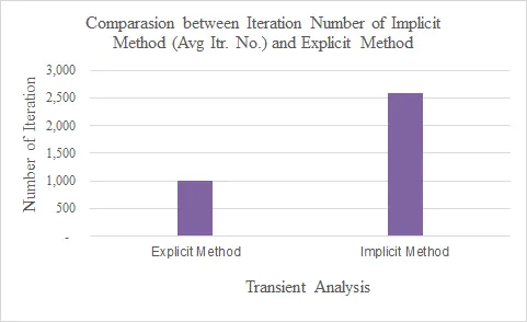
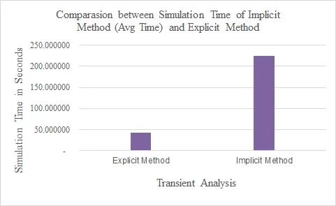
Based on CFL = 0.5 the following comparison has been done between implicit and explicit methods.

Discussion of Results:

1. In case of both Implicit Transient and Steady-state SOR converges faster than others. SOR> GS > Jacobi. This can well be understood by the iteration number and simulation time.

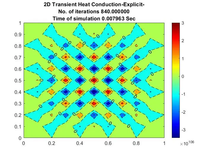
2. Between Implicit and Explicit methods of Transient, there is a limitation of explicit methods on the CFL number. The solutions blow up for CFL number greater than 0.5. The below mentioned one for CFL = 0.6

3. Between the fastest method of the steady-state and transient that is SOR, steady-state converges faster than transient.