Week 7 - Simulation of a 1D Super-sonic nozzle flow simulation using Macormack Method
AIM: To simulate the isentropic flow through a quasi 1D subsonic-supersonic nozzle.
INTRODUCTION:
In this project we are required to simulate isentropic flow through the nozzle using the MacCormack Method. Prior to dwelling deep into the MacCormack method, we shall understand what do subsonic and super sonic flows mean.
Subsonic Flow: The flow of a fluid is said to subsonic when the speed of flow is in the range of 0-0.9 Mach.
(where 1 Mach is the speed of sound)
Supersonic Flow: The flow of a fluid is said to subsonic when the speed of flow is greater than Mach 1.
The MacCormack Method and the Governing Equations:
The MacCormack method is an explicit finite difference method which is second order accurate. This method is a derivative of the much complex method the Lax Wendroff method. In this problem, we assume one end of the convergent-divergent nozzle is connected to a reservoir(ie. at inlet) where the speed of flow is considered nearly non existant. It is also assumed that the speed of the fluid is exactly Mach 1 at the throat and the area of cross-section is minimum.
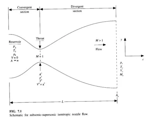
The MacCormack method comprises of two steps. Namely, the predictor step and the corrector step.
Predictor Step: In this step, we estimate the values of the primitive terms using Forword differencing.
Corrector Step: In this step, we correct the previously obtained values from the predictor step. To achieve this we use the backward differencing scheme.
Governing Equations:
The basic governing equations in CFD are the continuity, momentum and energy equations. The governing equations are usually written in 2 ways, namely, the conservation form and the non-conservation form. From the mathematical perspective they look quite similar with minute differences.
Non-Conservation Form:
Below are the equations for the continuity, momentum and energy.
CONTINUITY EQUATION:
`(del rho')/(del t') =-rho' (delV)/(del x') -rho' V' (lnA')/(delx') -V' (del rho')/(del x')`
MOMENTUM EQUATION:
`(delV')/(delt')=-V' (delV')/(delx') -1/gamma ((delT')/(delx')+ (T')/(rho') (del rho')/(del x'))`
ENERGY EQUATION:
`(delT')/(delt')= -V' (delT')/(del x')- (gamma-1) T' [(delV')/(delx')+ (del(lnA'))/(delx')]`
Initial conditions:

Conservation Form:
Below are the equations for the continuity, momentum and energy.
CONTINUITY EQUATION:
`(del (rho' A'))/(delt') + (del( rho' A' V'))/(delx')`
MOMENTUM EQUATION:
`(del(rho'A'V'))/(delt') +del[ (rho'A'V' + 1/gamma rho'A')/(del x')]=1/gamma rho' (delA')/(delx')`
ENERGY EQUATION:
`del[(rho' ((e')/(gamma-1) +gamma/2 (V')^2)A']/(delt')] + del[(rho' ((e')/(gamma-1) +gamma/2 (V')^2)V'A' +rho'A'V']/(delx')]=0`
The simplified version of the above is given below:
Solution vectors
`U_1=rho' A'`
`U_2=rho'A'V'`
`U_3= rho' ((e')/(gamma-1)+gamma/2 (V')^2)A'`
Pure Flux Terms:
`F_1=rho'A'V'`
`F_2=rho'A'(V')^2 +1/gamma rho'A'`
`F_3=rho' ((e')/(gamma-1)+gamma/2 (V')^2)V'A'+rho'A'V'`
Source term:
`J_2= 1/gamma rho' (delA')/(delx')`
GOVERNING EQUATIONS IN THE SIMPLIFIED FORM:
Continuity: `(delU_1)/(delt')=-(delF_1)/(delx')`
Momentum: `(delU_2)/(delt')=-(delF_2)/(delx') +J_2`
Energy: `(delU_3)/(delt')=-(delF_3)/(delx')`
Initial conditions
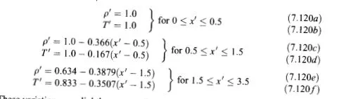
The above used terms such as x', T',`rho'`etc are all non dimensional forms of the primitive variables
TIMESTEP CALCULATION:
The time step is controlled by the Courant Friedrichs-Lowry ( CFL) criterion. We use this criterion to ensure that the solution to this problem remains stable. The criterion is `C<=1`. For this reason, I had chosen the value of C to be 0.5. The value of dt is determined by the following formula.
`Delta t= C (Deltax)/(a+v)`
With the above formula, we calculate the `Delta t` at each node. The value of `Delta t` is determined by simply considering the minimum value of `Delta t` obtained.
`Delta t= "minimum"((Deltat_1)^t +(Deltat_2)^t +(Deltat_3)^t+.............+(Deltat_N)^t )`
MAIN CODE:
Below is the code for simulating the quasi 1D subsonic-supersonic nozzle. This code has 2 functions inorder to maintain modularity.
- consevation_form.m
- nonconservative.m
Main Code:
 clear all
 close all
 clc

 %inputs
 n=31
 x=linspace(0,3,n);
 dx=x(2)-x(1);
 gamma=1.4;
 throat=((n-1)/2)+1;
 nt=1400;
%area
 a= 1+(2.2*(x-1.5).^2);

 %non conservation_form
 tic
 [rho,t,v,mass_flow_rate_non_con,mach_nc,P,mass_flow_rate_non_con_t,mach_nc_t,P_nc_t]=non_conservative(n,x,dx,a,gamma,nt,throat,a);
 time_nc=toc

 %conservation_form
 tic
 [rho_con,t_con,v_con,mfr_c,mach_c,P_c,mfr_t,mach_t,P_t]=conservation_form(n,x,dx,a,gamma,nt,throat) ;
 time_c=toc
 for e=1:n
  analytical_mfr(e)=0.579;
 end


 figure(5)
 plot(x,mass_flow_rate_non_con,'linewidth',1.5);
 hold on;
 plot(x,mfr_c,'linewidth',1.5);
 hold on;
 plot(x,analytical_mfr,'linewidth',1.5);
 grid minor
 xlabel('length of nozzle','fontsize',10);
 ylabel('mass flow rate',"fontsize",10);
 legend("non conservative","conservative","exact",'location','northeastoutside');
 title(" Variation of MFR in conservative, non-conservative and exact vs non-dimensional length",'fontsize',12);

 %comparison plots of primitive variables

 figure(6)
 %density
 subplot(4,1,1)
 plot(x,rho,'b','linewidth',1.5);
 hold on;
 plot(x,rho_con,'color','r','--','markersize',3);
 xlabel('length of nozzle','fontsize',10);
 ylabel('Density','fontsize',10);
 legend('non-conservative','conservative','location','northeastoutside')
 title('Density','fontsize',12,'fontweight','bold');
 grid minor

% temperature
 subplot(4,1,2)
 plot(x,t,'b','linewidth',1.5);
 hold on;
 plot(x,t_con,'color','r','--','markersize',3);
 xlabel('length of nozzle','fontsize',10);
 ylabel('temperature','fontsize',10);
 legend("non-conservative","conservative",'location','northeastoutside')
 title('Temperature','fontsize',12,'fontweight','bold');
 grid minor

 %mach number
 subplot(4,1,3)
 plot(x,mach_nc,'b','linewidth',1.5);
 hold on;
 plot(x,mach_c,'color','r','--','markersize',3);
 xlabel('length of nozzle','fontsize',10);
 ylabel('mach number','fontsize',10);
 legend("non-conservative","conservative",'location','northeastoutside')
 title('Mach Number','fontsize',12,'fontweight','bold');
 grid minor

 %pressure
 subplot(4,1,4)
 plot(x,P,'b','linewidth',1.5);
 hold on;
 plot(x,P_c,'color','r','--','markersize',3);
 xlabel('length of nozzle','fontsize',10);
 ylabel('pressure','fontsize',10);
 legend("non-conservative","conservative",'location','northeastoutside');
 title('Pressure','fontsize',12,'fontweight','bold');
 grid minor
Non Conservative Form:
## clear all
## close all
## clc
##
## %inputs
## n=31
## x=linspace(0,3,n);
## dx=x(2)-x(1);
## gamma=1.4;
## throat=((n-1)/2)+1;
function [rho,t,v,mass_flow_rate_non_con,mach_nc,P,mass_flow_rate_non_con_t,mach_nc_t,P_nc_t]=non_conservative(n,x,dx,a,gamma,nt,throat,area)
 %calculate initial profiles at T=0(time)
 rho=1-(0.3146*x);
 t=1-(0.2314*x ) ;  %t=temp
 v=(0.1+(1.09*x)).*(t.^0.5);
 %throat =((n-1)/2)+1;

## %area
## a= 1+(2.2*(x-1.5).^2);


 % Time steps
 nt=1400;
 c=0.5 %courant number

 dt_a=((c*dx)./((t.^0.5)+v));

 dt_nc=min(dt_a)
 rho_ini=rho;
   v_ini=v;
   t_ini=t;

 %outer time loop
 for k=1:nt
   %predictor methods
   %continuity eqn
   rho_old=rho;
   v_old=v;
   t_old=t;

   %predictor methods
   %continuity eqn
   for j= 2:n-1
    %drho_dt_p=-tho(j)*(v(j+1)-v(j))/dx-rho(j)*v(j)*(log(a(j+1))-log(a(j)))/dx
    dvdx=(v(j+1)-v(j))/dx;
    drhodx= (rho(j+1)-rho(j))/dx;
    dtdx=(t(j+1)-t(j))/dx;
    dlogadx=(log(a(j+1))-log(a(j)))/dx;
    %continuity
    drho_dt_p(j)= -rho(j)*dvdx -rho(j)*v(j)*dlogadx -v(j)*drhodx;

    %momentum
    dvdt_p(j)= -v(j)*dvdx -(1/gamma)*(dtdx + (t(j)/rho(j))*drhodx);

    %energy eqn
    dtdt_p(j)= -v(j)*dtdx - (gamma-1)*t(j)*(dvdx + v(j)*dlogadx);

    %solution update
    rho(j)=rho(j)+drho_dt_p(j)*dt_nc;
    v(j)=v(j)+dvdt_p(j)*dt_nc;
    t(j)=t(j)+dtdt_p(j)*dt_nc;
  end

    %corector methods
   %
   for i= 2:n-1
    %drho_dt_p=-tho(j)*(v(j+1)-v(j))/dx-rho(j)*v(j)*(log(a(j+1))-log(a(j)))/dx
    dvdx=(v(i)-v(i-1))/dx;
    drhodx= (rho(i)-rho(i-1))/dx;
    dtdx=(t(i)-t(i-1))/dx;
    dlogadx=(log(a(i))-log(a(i-1)))/dx;
    %continuity
    drho_dt_c(i)= -rho(i)*dvdx -rho(i)*v(i)*dlogadx -v(i)*drhodx;

    %momentum
    dvdt_c(i)= -v(i)*dvdx -(1/gamma)*(dtdx + (t(i)/rho(i))*drhodx);

    %energy eqn
    dtdt_c(i)= -v(i)*dtdx - (gamma-1)*t(i)*(dvdx + v(i)*dlogadx);

  end

  %compute the average derivative
  drhodt= 0.5*(drho_dt_p + drho_dt_c);
  dvdt= 0.5*(dvdt_p + dvdt_c);
  dtdt= 0.5*(dtdt_p+dtdt_c);

  %final update
  for l=2:n-1

    rho(l)= rho_old(l)+drhodt(l)*dt_nc;
    v(l)=v_old(l)+dvdt(l)*dt_nc;
    t(l)=t_old(l)+dtdt(l)*dt_nc;

  end

  %inlet conditions
  v(1)=2*v(2) - v(3);
  %rho(1)=2*rho(2)-rho(3);
  %t(1)=2*t(2)-t(3);


  %outlet conditions
  v(n)=2*v(n-1) - v(n-2);
  rho(n)=2*rho(n-1) - rho(n-2);
  t(n)=2*t(n-1) - t(n-2);

  mass_flow_rate_non_con=rho.*v.*a;
  mach_nc=v./(t.^0.5);
  P=rho.*t;

  % at throat
  v_nc_t(k)=v(throat);
  rho_nc_t(k)=rho(throat);
  t_nc_t(k)=t(throat);
  mass_flow_rate_non_con_t(k)=mass_flow_rate_non_con(throat);
  mach_nc_t(k)=mach_nc(throat);
  P_nc_t(k)=P(throat);


 figure(1)
    hold all;
    if k==50
      plot(x,mass_flow_rate_non_con,'k');


    elseif k==100
     plot(x,mass_flow_rate_non_con,'c');


    elseif k==200
     plot(x,mass_flow_rate_non_con,'g');


  elseif k==600
    plot(x,mass_flow_rate_non_con,'b');

  elseif k==800
     plot(x,mass_flow_rate_non_con,'r');

   elseif k==1400
     plot(x,mass_flow_rate_non_con,'m');

     end


  end


   title("Variation of mass flow rate vs length of nozzle for non conservative form and time steps","fontsize",12)
   legend('50','100','200','600','800','1400')
   grid minor
   xlabel("length of nozzle","fontsize",10)
   ylabel("mass flow rate","fontsize",10)

  figure(4)
    %plot for density at throat
    X=linspace(1,nt,nt);

    subplot(2,2,1)

    plot(X,rho_nc_t,'k');
    hold on;
    title({["non conservation form"];["Variation of density VS Timesteps"]},"fontsize",12);
    xlabel("timesteps","fontsize",10)
    ylabel("density","fontsize",10)
    grid minor

    %plot for temperature
    subplot(2,2,2)

    plot(X,t_nc_t,'b');
    hold on;
    xlabel("timesteps","fontsize",10);
    ylabel("temperature","fontsize",10);
    title({["non conservation form"];["Variation of temperature VS Timesteps"]},"fontsize",12);
    grid minor

   % Mach number
   subplot(2,2,3)

   plot(X,mach_nc_t,'g');
   xlabel("timesteps","fontsize",10);
   ylabel("mach number","fontsize",10);
   title({["non conservation form"];["Variation of mach number VS Timesteps"]},"fontsize",12);
   grid minor

   %pressure
   subplot(2,2,4)

   plot(X,P_nc_t,"r");
   xlabel("timesteps","fontsize",10);
   ylabel("pressure","fontsize",10);
   title({["non conservation form"];["Variation of pressure VS Timesteps"]},"fontsize",12);
   grid minor


end
Conservative Form:
##  conservation format
##
## clear all
## close all
## clc
##
## n=31
## x=linspace(0,3,n);
## dx=x(2)-x(1);
## gamma=1.4
## throat=((n-1)/2)+1;
function [rho_con,t_con,v_con,mfr_c,mach_c,P_c,mfr_t,mach_t,P_t]=conservation_form(n,x,dx,a,gamma,nt,throat)
  for i = 1:n
     if ( 0<=x(i) && x(i)<=0.5)
       rho_con(i)=1;
       t_con(i)=1;

     elseif (x(i)>=0.5 && x(i)<=1.5)
       rho_con(i)=1.0-(0.366*(x(i)-0.5));
       t_con(i)=1.0-(0.167*(x(i)-0.5));

     elseif( x(i)>=1.5 && x(i)<=3)
       rho_con(i)=0.634-(0.3879*(x(i)-1.5));
       t_con(i)=0.833-(0.3507*(x(i)-1.5));

    end

 end

## %area
## a= 1+(2.2*(x-1.5).^2);


 %velocity
 v_con=0.59./(rho_con.*a);
 pr_con=rho_con.*t_con;
 u1=rho_con.*a;
 u2=rho_con.*a.*v_con;
 u3=u1.*(((t_con)/(gamma-1))+(gamma/2).*(v_con.^2));

 % time
 c=0.5
 throat =((n-1)/2)+1;
 dt_a=(c*dx)./((t_con.^0.5)+v_con);

 dt=min(dt_a);
%dt = 0.0267; %Value used in Anderson, for validation.

 nt=1400;
   u1_ini=u1;
   u2_ini=u2;
   u3_ini=u3;
 for i=1:nt

##    dt_a=c*((dx)./((t_con.^0.5)+v_con));

    #dt=min(dt_a);
   % storing old values of the solution vectors
   u1_old=u1;
   u2_old=u2;
   u3_old=u3;

   %pure flux terms
   f1=u2;
   term1= ((gamma-1)/gamma)*(u3 - (gamma*u2.^2)./(2*u1));
   f2=((u2.^2)./u1) + term1;
   term2=((gamma*(gamma-1))*(u2.^3))./(2*u1.^2);
   f3=((gamma*u2.*u3)./u1)-term2;


   %predictor method
   for j=2:n-1
     df1dx(j)=(f1(j+1)-f1(j))/dx;
     df2dx(j)=(f2(j+1)-f2(j))/dx;
     df3dx(j)=(f3(j+1)-f3(j))/dx;

     dadx(j)=(a(j+1)-a(j))/dx;

     j2(j)=(1/gamma)*(rho_con(j).*t_con(j).*dadx(j));

     %continuity
     du1dt_p(j)= -df1dx(j);

     %momentum
     du2dt_p(j)= - df2dx(j)+j2(j);

     %energy
     du3dt_p(j)= -df3dx(j);


     %solution update
     u1(j)=u1(j)+du1dt_p(j)*dt;
     u2(j)=u2(j)+du2dt_p(j)*dt;
     u3(j)=u3(j)+du3dt_p(j)*dt;

   end


   %Decoding the primitive variables
   rho_con=u1./a;
   v_con=u2./u1;
   t_con=(gamma-1)*((u3./u1)-(gamma/2)*v_con.^2);


   %pure flux terms
   f1=u2;
   term1= ((gamma-1)/gamma)*(u3 - (gamma/2)*(u2.^2/u1));
   f2=((u2.^2)./u1) + term1;
   term2=((gamma*(gamma-1))/2)*(u2.^3./u1.^2);
   f3=gamma*((u2.*u3)./u1)-term2;
##
##


   %corrector step

   for k=2:n-1
     df1dx(k)=(f1(k)-f1(k-1))/dx;
     df2dx(k)=(f2(k)-f2(k-1))/dx;
     df3dx(k)=(f3(k)-f3(k-1))/dx;

     dadx(k)=(a(k)-a(k-1))/dx;

     j2(k)=(1/gamma)*(rho_con(k).*t_con(k).*dadx(k));

     %continuity
     du1dt_c(k)= -df1dx(k);

     %momentum
     du2dt_c(k)= -df2dx(k)+j2(k);

     %energy
     du3dt_c(k)= -df3dx(k);


   end

   %average derivative

   du1dt=0.5*(du1dt_p+du1dt_c);
   du2dt=0.5*(du2dt_p+du2dt_c);
   du3dt=0.5*(du3dt_p+du3dt_c);
##
   %final update
   for k=2:n-1
     u1(k)= u1_old(k)+du1dt(k)*dt;
     u2(k)= u2_old(k)+du2dt(k)*dt;
     u3(k)= u3_old(k)+du3dt(k)*dt;
   end

   % inlet conditions

   %constant as rho is fixed as it is independant of time
   u1(1)=rho_con(1)*a(1);  %% ERROR LHS is U(1) and not U

   %Floating term can be found by extrapolation of u2
   u2(1)=2*u2(2)-u2(3);

   %used to find value of u3 at node 1 sinve v is floating
   v_con(1)=u2(1)/u1(1); %% ERROR Variable v_con should be used and not just v

   %finding u3
   u3(1)=u1(1)*((t_con(1)/(gamma-1))+((gamma/2)*v_con(1)^2));


   % final conditions
   u1(n)=2*u1(n-1)-u1(n-2);
   u2(n)=2*u2(n-1)-u2(n-2);
   u3(n)=2*u3(n-1)-u3(n-2);

   %Decoding the primitive variables
   rho_con=(u1)./a;
   v_con=u2./u1;
   t_con=(gamma-1).*((u3./u1)-(gamma/2)*v_con.^2);

   %solutions
    mfr_c=rho_con.*v_con.*a;
    mach_c=v_con./(t_con.^0.5);
    P_c=rho_con.*t_con;

   % values at throat
   rho_t(i)=rho_con(throat);
   v_t(i)=v_con(throat);
   t_t(i)=t_con(throat);
   mfr_t(i)=mfr_c(throat);
   mach_t(i)=mach_c(throat);
   P_t(i)=P_c(throat);

   figure(2)
   hold all;
   if i==100
      plot(x,mfr_c,'k');


   elseif i==200
     plot(x,mfr_c,'c');


   elseif i==700
     plot(x,mfr_c,'g');


   elseif i==1000
     plot(x,mfr_c,'b');

    end


end
  grid minor
   title("variation of mass flow rate vs length of nozzle","fontsize",12)
   legend('100','200','700','1000')
   ylabel("mass flow rate","fontsize",10)
   xlabel("length of nozzle","fontsize",10)
    X=linspace(1,nt,nt);

    figure(3)
    %plot for density at throat


    grid minor
    subplot(2,2,1)

    plot(X,rho_t,'k');
    hold on;
    xlabel("timesteps")
    ylabel("density")
    title({[" conservation form"];["Variation of density VS Timesteps at throat"]});
    grid minor

    %plot for temperature
    subplot(2,2,2)

    plot(X,t_t,'b');
    hold on;
    xlabel("timesteps");
    ylabel("temperature");
    title({[" conservation form"];["Variation of temperature VS Timesteps at throat"]});
    grid minor
    % Mach number
   subplot(2,2,3)

   plot(X,mach_t,'g');
   xlabel("timesteps");
   ylabel("mach number");
   title({[" conservation form"];["Variation of mach number VS Timesteps at throat"]});
   grid minor

   %pressure
   subplot(2,2,4)

   plot(X,P_t,"r");
   xlabel("timesteps");
   ylabel("pressure");
   title({[" conservation form"];["Variation of pressure VS Timesteps at throat"]});
   grid minor
   end
RESULTS:
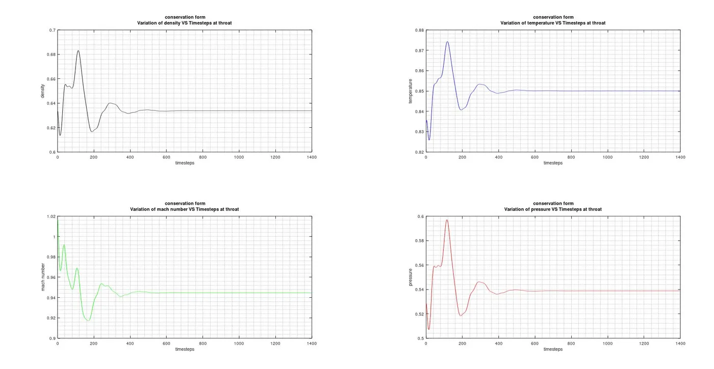
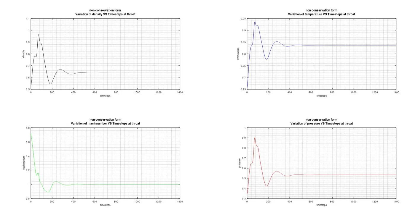
Timestep wise variation of primitive variables at throat:
CONSERVATION FORM:
NON-CONSERVATION FORM:
Inference:
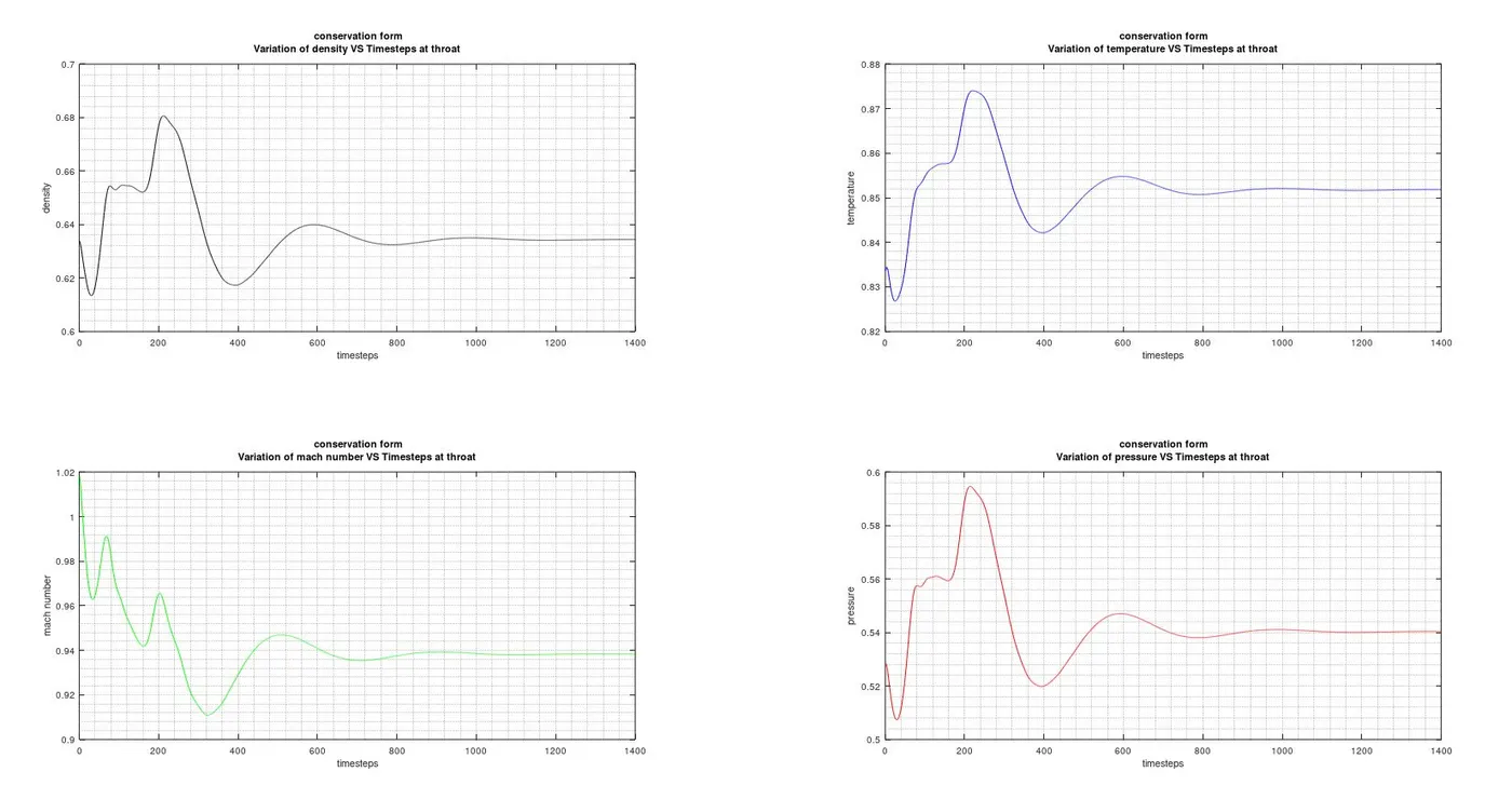
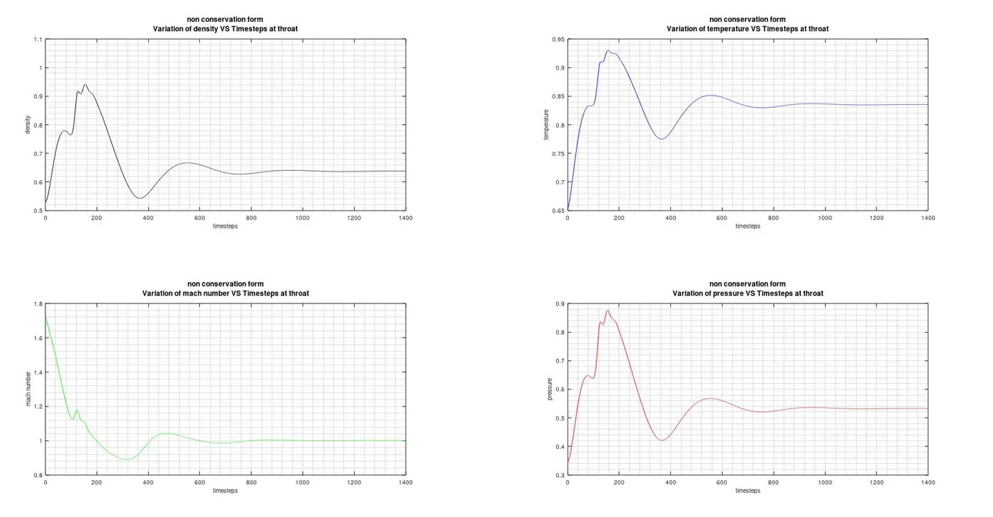
From the above plots, we can infer that the primitive variables attain stability quicker in the conservation method compared to the latter. This also implies that the time wise variation in the former is less compared to the latter.
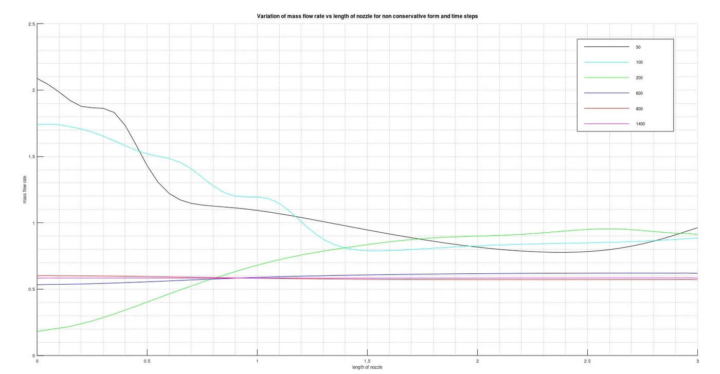
INSTANTANEOUS DISTRIBUTION OF MASS FLOW RATE:
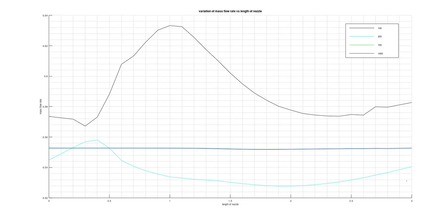
CONSERVATION FORM:
NON-CONSERVATION FORM:
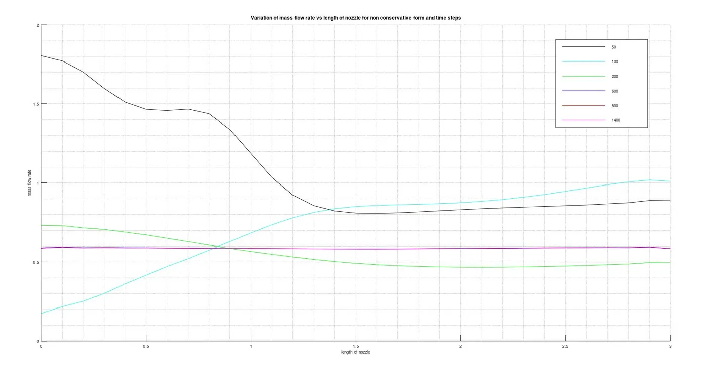
Inference:
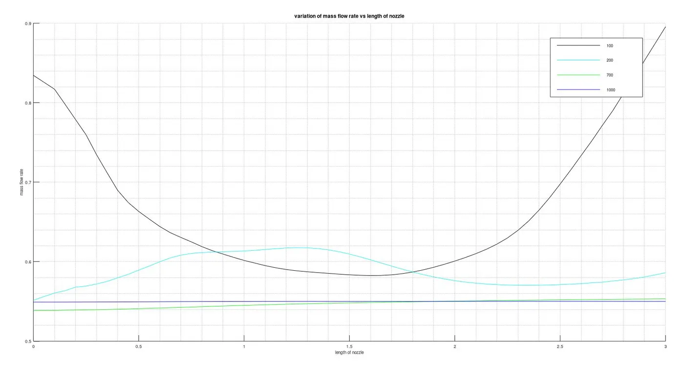
In both cases the mass flow rate variation oscillates for the first few time steps (approx till 500) post this, the solution is observed to be stable.
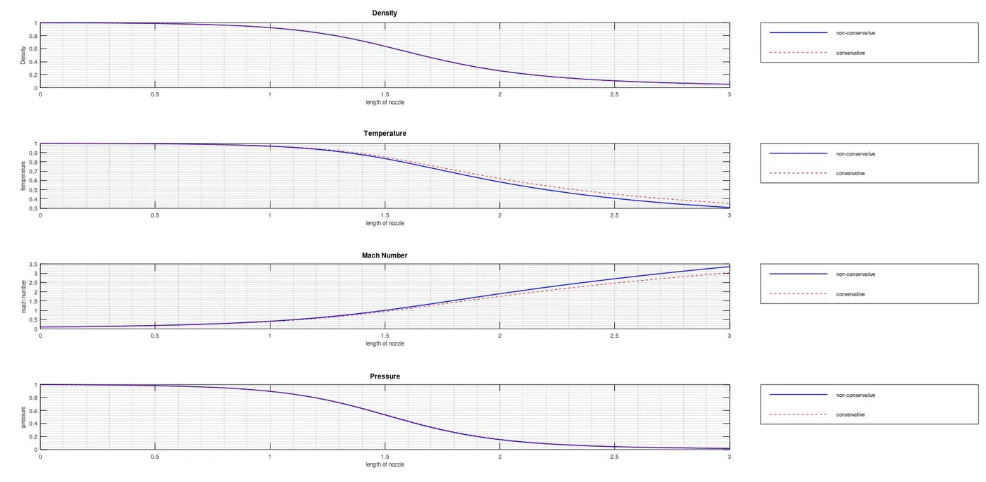
COMPARISON PLOT OF VARIATION OF PRIMITIVE VARIABLES WITH RESPECT TO LENGTH IN BOTH FORMS:
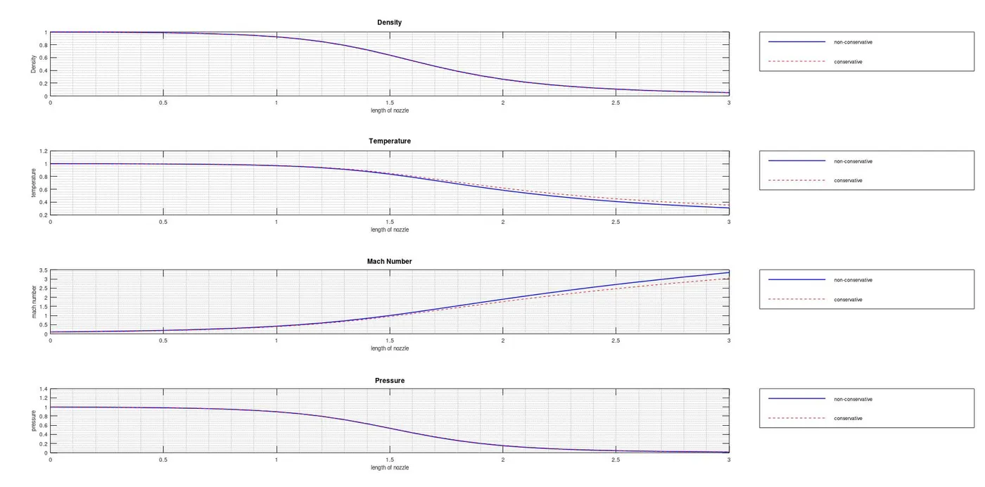
Inference:
From the above plots, we can infer that the variation of the primitive variables in both forms are not very significant. They almost follow the same paths.
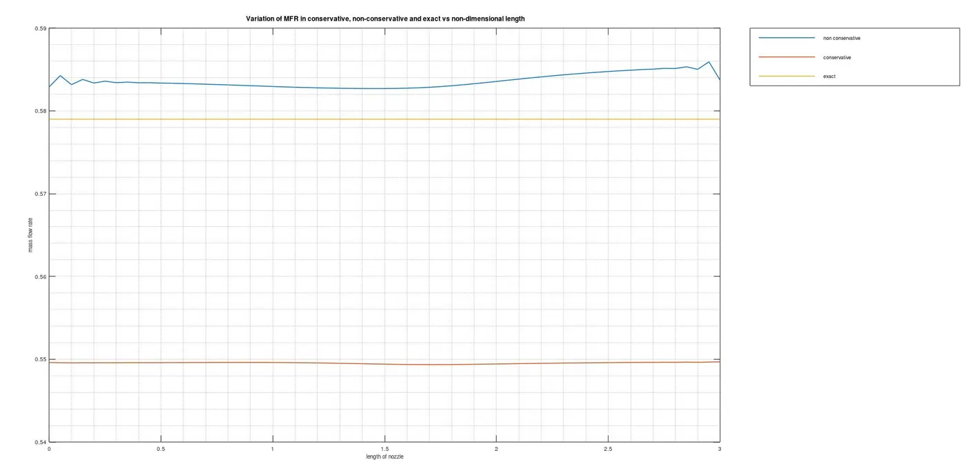
NORMALIZED MASS FLOW RATE PLOT:
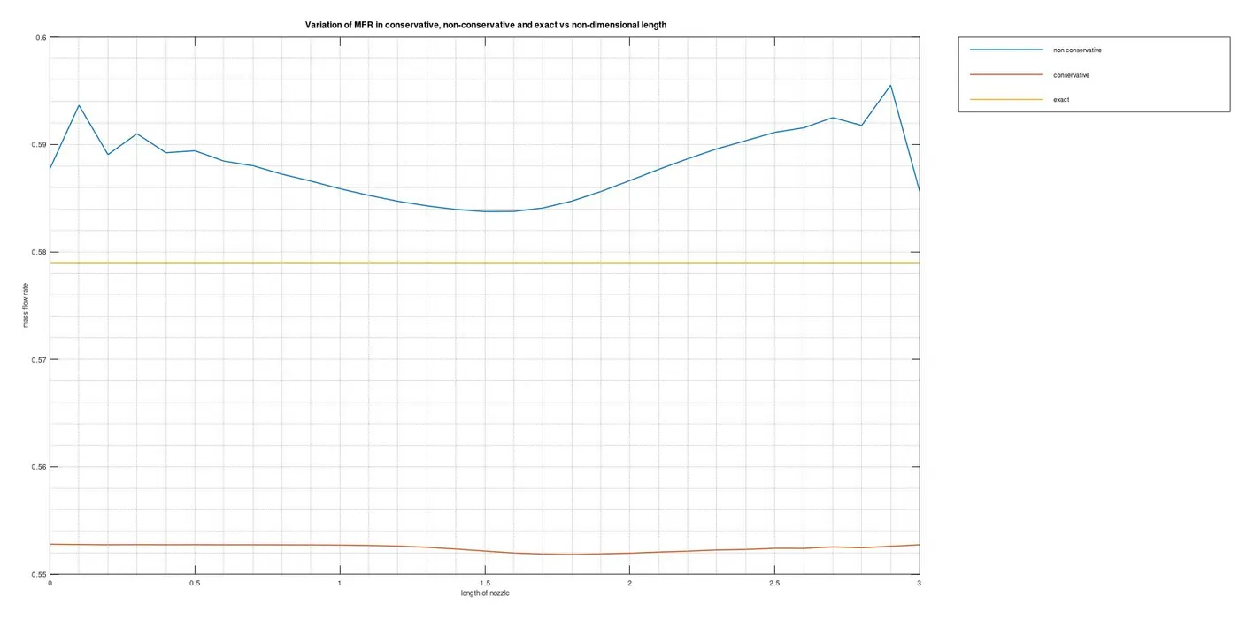
Inference:
From the above plots, we can infer that the conservative method attains stability sooner than the non-conservation method. Also the oscillation at the onlet and outlet for the non-conservative method are significant, whereas in the latter is almost linear with least deviations.
GRID INDEPENDANCE TEST:
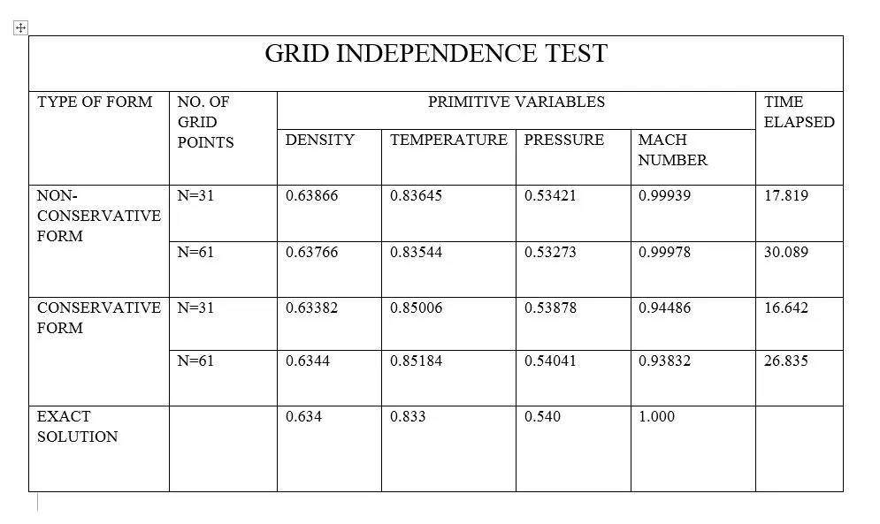
Inference:
Above is a tabulation of the values of the primitive variables when computed for grid sizes n=31 and n=61. From the above results, we can observe that in either case, the values of the primitive variables are quite similar. However, we can observe a marginal improvement when the gird points was increased to n=61. Since the increase is very minute and all the methods yield solutions close to the exact solution, it is safe to say that this problem is grid independant.
PLOTS FOR N=61:
Timestep wise variation of primitive variables at throat:
CONSERVATION FORM:
NON-CONSERVATION FORM:
INSTANTANEOUS DISTRIBUTION OF MASS FLOW RATE:
CONSERVATION FORM:
NON-CONSERVATION FORM:
COMPARISON PLOT OF VARIATION OF PRIMITIVE VARIABLES WITH RESPECT TO LENGTH IN BOTH FORMS:
NORMALIZED MASS FLOW RATE PLOT:
CONCLUSION:
- When we consider accuracy, both the methods almost yield similar results. Interms of accuracy we may say that the non-conservative method has a slight edge over the latter.
- The non-conservative method gives us residual.
- The conservative method was found to be the fastest in computational time in spite of it being complex.
- The conservative method attains stability much quicker compared to the other method. It was also the most stable compared to the latter.
- The solutions in either case are close to the actual values.
- This problem is GRID INDEPENDANT.
REFERENCES:
Computational Fluid Dynamics- with basics and application- John D Anderson.