Simulation of Quasi 1-D Supersonic Nozzle Flow Using MacCormack Method
Objective: To find the -
- Steady-state distribution of primitive variables inside the nozzle.
- Time-wise variation of the primitive variables.
- Variation of Mass flow rate distribution inside the nozzle at different time steps during the time-marching process.
- Comparison of Normalized mass flow rate distributions of both forms.
- Grid Dependence Test.
These will be done by solving the governing equations in both conservative and non-conservative forms.
Theory:
We consider the steady, isentropic flow through a convergent-divergent nozzle. The flow at the inlet to the nozzle comes from a reservoir where the pressure and temperature are denoted by `p_0` , and `T_0`, respectively. The cross-sectional area of the reservoir is large ( `A -> infty` ), and hence the velocity is very small (`V -> 0` ). Thus, `p_0` and `T_0` are the stagnation values, or total pressure and total temperature, respectively. The flow expands isentropically to supersonic speeds at the nozzle exit. The flow is locally subsonic in the convergent section of the nozzle, sonic at the throat (minimum area), and supersonic at the divergent section. The sonic flow (M = 1) at the throat means that the local velocity at this location is equal to the local speed of sound.
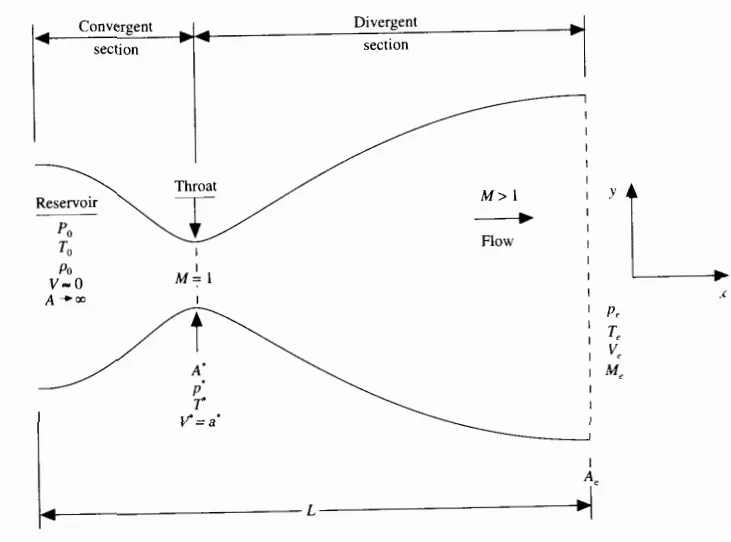
The variables have been non-dimensionalised as:-
`T' = T/T_0` , `rho' = rho/rho_0`, `x' = x/L`, `V' = V/a_0` where `a_0 = sqrt(gammaRT_0)`, `t' = t/(L/a_0)`, `A' = A/(A^ast)` where `A^ast` is the area of the nozzle at the throat, R is universal gas constant, and gamma is the ratio of specific heats.
1.Conservative form:
a. Governing equations:
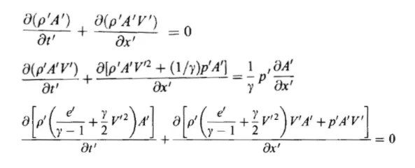
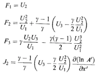
These equations are transformed by grouping variables into solution vectors(`U_1,U_2,U_3`), flux vectors(`F_1,F_2,F_3`) and source term(`J_2`).
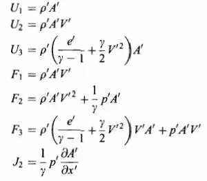
With these definitions in place, the governing equations can also be written as :-
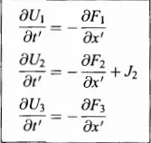
By solving these equations, we would be solving for the solution vectors, and not for the primitive variables like density, termperature, pressure, velocity. Thus, it is necessary to write the flux vectors and source term in terms of the solution vector for numerical analysis.
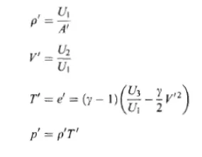
From here, the primitive variables can be written as:-
b. Boundary Conditions:
At inlet boundary,
`U_{1(i=1)} = rho'_{(i=1)}*A'_{(i=1)}`
`U_{2(i=1)} = 2U_{2(i=2)} - U_{2(i=3)}`
`U_3 = U_1(T/(gamma-1) + (gamma/2)V'^2)`
At outlet boundary,
`U_{1(n)} = 2U_{1(n-1)} - U_{1(n-2)}`
`U_{2(n)} = 2U_{2(n-1)} - U_{2(n-2)}`
`U_{3(n)} = 2U_{3(n-1)} - U_{3(n-2)}`
c. Initial Conditions:
Area of the nozzle is constant and invariant with time. Considering a constant mass flow through the nozzle, initial velocity is assumed to be,
`V' = 0.59/(rho'A')`
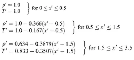
At t'=0, value of density and temperature throughout the nozzle is given as follows-
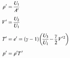
After the calculation of the solution vectors, the primitive variables can be calculated by the equations-
2. Non-Conservative form:
a. Governing equations:



b. Boundary conditions:
At inlet boundary,
Velocity is changing with time as density and temperature are constant at their respective stagnation values.
`V_1 = 2V_2 - V_3`
At outlet boundary,
`V_{n} = 2V_{n-1} - V_{n-2}`
`rho_{n} = 2rho_{n-1} - rho_{n-2}`
`T_{n} = 2T_{n-1} - T_{n-2}`
c. Initial conditions:
Area of the nozzle is constant with time.

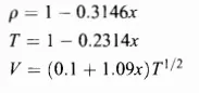
The flow field variables vary with respect to time.
The MacCormack method:
The MacCormack technique is a widely used discretixation scheme used for the solution of hyperbolic partial differential equations. This method is second-order accurate in both time and space.
Consider the following hyperbolic PDE,
`(delu)/(delt) = (delv)/(delx)`
The equation is solved in 2 steps, namely the predictor step and the corrector step.
Predictor step - The space derivative is forward differenced at the time step n, to give a value of u at the (n+1)th time step. The values at the nth time step are known.
`((delu)/(delt))_p =(v_{i+1}^n - v_i^n)/(Deltax)`
This derivative is used to compute the predicted value of u at the (n+1)th time step.
`u_i^(n+1) = u_i^n + ((delu)/(delt))_p*Deltat`
This predicted value is used for the corrector step which uses backward differences for space derivatives.
`((delu)/(delt))_c =(v_{i}^n - v_{i-1}^n)/(Deltax)`
The two derivatives are used to calculate the average derivative and used to compute the final value of u at the (n+1)th time step.
`((delu)/(delt))_{avg} = 0.5(((delu)/(delt))_p + ((delu)/(delt))_c)`
`u_i^(n+1) = u_i^n + ((delu)/(delt))_{avg}*Deltat`. This gives the final value of u at the (n+1)th time step.
The same method is repeated for all the internal grid points that the nozzle has been divided into, for 1400 time steps.
Calculation of time step:
In order to have a stable solution, the Courant number cannot exceed 0.5 for a hyperbolic PDE.
From this consider, we can calculate the value of time step that can be used for a stable solution.
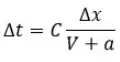 where C is Courant number, V is local velocity of fluid, a is local speed of sound, `Deltax` is length of grid.
According to the value in John D. Anderson textbook, a step of dt = 0.0267 has been used for solution.
Matlab Script:
Non-Conservative form:
%Non-Conservation Code
clear all
close all
clc

%Inputs
n = 31;
x = linspace(0,3,n);
dx = x(2)-x(1);

%Initial profiles
rho = 1-0.3146*x;
T = 1-0.2314*x;
v = (0.1+1.09*x).*T.^0.5;
A = 1+2.2*(x-1.5).^2;
gamma = 1.4;

%time steps
nt = 1400;
dt = 0.0267;

%Outer time loop
for k=1:nt

    %Predictor step
    rho_old = rho;
    v_old = v;
    T_old = T;
    %Space loop
    for j=2:n-1
        dvdx = (v(j+1)-v(j))/dx;
        drhodx = (rho(j+1)-rho(j))/dx;
        dTdx = (T(j+1)-T(j))/dx;
        dlogAdx = (log(A(j+1))-log(A(j)))/dx;
        %Continuity Eqn
        drhodt_p(j) = -rho(j)*dvdx - rho(j)*v(j)*dlogAdx - v(j)*drhodx;
        %Momentum Eqn
        dvdt_p(j) = -v(j)*dvdx - (1/gamma)*(dTdx + (T(j)/rho(j))*drhodx);
        %Energy Eqn
        dTdt_p(j) = -v(j)*dTdx - (gamma-1)*T(j)*(dvdx + v(j)*dlogAdx);

        %Solution update
        rho(j) = rho(j) + drhodt_p(j)*dt;
        v(j) = v(j) + dvdt_p(j)*dt;
        T(j) = T(j) + dTdt_p(j)*dt;

    end

    %Corrector step
    %Space loop
    for j=2:n-1
        dvdx = (v(j)-v(j-1))/dx;
        drhodx = (rho(j)-rho(j-1))/dx;
        dTdx = (T(j)-T(j-1))/dx;
        dlogAdx = (log(A(j))-log(A(j-1)))/dx;
        %Continuity Eqn
        drhodt_c(j) = -rho(j)*dvdx - rho(j)*v(j)*dlogAdx - v(j)*drhodx;
        %Momentum Eqn
        dvdt_c(j) = -v(j)*dvdx - (1/gamma)*(dTdx + (T(j)/rho(j))*drhodx);
        %Energy Eqn
        dTdt_c(j) = -v(j)*dTdx - (gamma-1)*T(j)*(dvdx + v(j)*dlogAdx);

    end

    %Compute average time derivative

    drhodt = 0.5*(drhodt_p + drhodt_c);
    dvdt = 0.5*(dvdt_p + dvdt_c);
    dTdt = 0.5*(dTdt_p + dTdt_c);

    %Final Solution update
    for i = 2:n-1
        rho(i) = rho_old(i) + drhodt(i)*dt;
        v(i) = v_old(i) + dvdt(i)*dt;
        T(i) = T_old(i) + dTdt(i)*dt;

    end

    %Boundary Conditions
    %Inlet
    v(1) = 2*v(2) - v(3);
    %Outlet
    v(n) = 2*v(n-1) - v(n-2);
    rho(n) = 2*rho(n-1) - rho(n-2);
    T(n) = 2*T(n-1) - T(n-2);

    p = rho.*T;
    M = v./sqrt(T);
    mflow = rho.*A.*v;

    %Values at throat
    th = find(A==1);
    p_th(k) = p(th);
    rho_th(k) = rho(th);
    T_th(k) = T(th);
    M_th(k) = M(th);

    figure(6)
     hold on
     if k==50
         plot(x,mflow,'r','linewidth',1.5);
     elseif k==100
         plot(x,mflow,'g','linewidth',1.5);
     elseif k==200
         plot(x,mflow,'c','linewidth',1.5);
     elseif k==700
         plot(x,mflow,'k','linewidth',1.5);
     end


end

%Exact solution
rho_exact = 0.634*ones(1,1400);
T_exact = 0.833*ones(1,1400);
p_exact = 0.528*ones(1,1400);
M_exact = 1*ones(1,1400);

%Convergence at throat
figure(1)
plot(1:nt,rho_th);
hold on
plot(1:nt,rho_exact);
legend('Non-Conservative form','Exact value');
xlabel('Length of nozzle');
ylabel('Density Ratio');
title('Variation of density');

figure(2)
plot(1:nt,p_th);
hold on
plot(1:nt,p_exact);
legend('Non-Conservative form','Exact value');
xlabel('Length of nozzle');
ylabel('Pressure Ratio');
title('Variation of pressure');

figure(3);
plot(1:nt,T_th);
hold on
plot(1:nt,T_exact);
legend('Non-Conservative form','Exact value');
xlabel('Length of nozzle');
ylabel('Temperature Ratio');
title('Variation of temperature');

figure(4)
plot(1:nt,M_th);
hold on
plot(1:nt,M_exact);
legend('Non-Conservative form','Exact value');
xlabel('Length of nozzle');
ylabel('Mach Number');
title('Variation of Mach Number');

figure(6)
title('Variation of mass flow rate with time');
xlabel('Length of nozzle');
ylabel('Mass flow rate');
legend('50dt','100dt','200dt','700dt','Location','best');

%Plots
 figure(5)
 subplot(2,2,1);
 plot(x,rho);
 grid on;
 xlabel('Length of nozzle');
 ylabel('Density Ratio');


 subplot(2,2,2);
 plot(x,M);
 grid on;
 xlabel('Length of nozzle');
 ylabel('Mach Number');


 subplot(2,2,3);
 plot(x,T);
 grid on;
 xlabel('Length of nozzle');
 ylabel('Temperature Ratio');


 subplot(2,2,4);
 plot(x,p);
 grid on;
 xlabel('Length of nozzle');
 ylabel('Pressure Ratio');

 suptitle('Variation of flow parameters across nozzle');
Conservative Form:
%Conservation Code

clear all
close all
clc

%Grid Spacing
n = 31;
x = linspace(0,3,n);
dx = x(2)-x(1);
gamma = 1.4;
nt = 1400;
%Initial profiles
for i=1:n
    if x(i)>=0 && x(i)<=0.5
        rho(i) = 1;
        T(i) = 1;
    elseif x(i)>=0.5 && x(i)<=1.5
        rho(i) = 1 - 0.366*(x(i) - 0.5);
        T(i) = 1 - 0.167*(x(i) - 0.5);
    elseif x(i)>=1.5 && x(i)<=3.5
        rho(i) = 0.634 - 0.3879*(x(i) - 1.5);
        T(i) = 0.833 - 0.3507*(x(i) - 1.5);
    end
end

%Initial conditions
A = 1+2.2*(x-1.5).^2;
v = 0.59./(rho.*A);
u1 = rho.*A; %Solution vector 1
u2 = rho.*A.*v; %Solution vector 2
u3 = u1.*((T./(gamma-1) + (gamma/2)*(v.^2))); %Solution vector 3
C = 0.5;
dt = 0.0267 %time step

%Time loop
for k=1:nt
    u1_old = u1;
    u2_old = u2;
    u3_old = u3;

    %Flux terms defined in terms of solution vectors
    f1 = u2;
    f2 = u2.^2./u1 + ((gamma-1)/gamma)*(u3 - (gamma/2)*(u2.^2./u1));
    f3 = (gamma*u2.*u3)./u1 - gamma*((gamma-1)/2)*(u2.^3./u1.^2);

    %Predictor step
    for j=2:n-1
        dadx = (A(j+1)-A(j))/dx;
        j2 = (1/gamma).*rho(j).*T(j).*dadx;

        %Continuity Equation
        du1dt_p(j) = -(f1(j+1) - f1(j))/dx;

        %Momentum Equation
        du2dt_p(j) = -(f2(j+1) - f2(j))/dx + j2 ;

        %Energy Equation
        du3dt_p(j) = -(f3(j+1) - f3(j))/dx;

        %Solution update
        u1(j) = u1(j) + du1dt_p(j)*dt;
        u2(j) = u2(j) + du2dt_p(j)*dt;
        u3(j) = u3(j) + du3dt_p(j)*dt;
    end

    %Predicting the primitives

    rho = u1./A;
    v = u2./u1;
    temp = (gamma-1)*(u3./u1 - (gamma/2)*v.^2);

    %Updating flux terms

    f1 = u2;
    f2 = u2.^2./u1 + ((gamma-1)/gamma)*(u3 - (gamma/2)*(u2.^2./u1));
    f3 = (gamma*u2.*u3)./u1 - gamma*((gamma-1)/2)*(u2.^3./u1.^2);

    %Corrector step
     for j=2:n-1
        dadx = (A(j)-A(j-1))/dx;
        j2 = (1/gamma).*rho(j).*T(j).*dadx;

        %Continuity Equation
        du1dt_c(j) = -(f1(j) - f1(j-1))/dx;

        %Momentum Equation
        du2dt_c(j) = -(f2(j) - f2(j-1))/dx + j2 ;

        %Energy Equation
        du3dt_c(j) = -(f3(j) - f3(j-1))/dx;

     end
     %Average time derivatives
     du1dt = 0.5*(du1dt_p + du1dt_c);
     du2dt = 0.5*(du2dt_p + du2dt_c);
     du3dt = 0.5*(du3dt_p + du3dt_c);

     %Solution Update
     for j=2:n-1
         u1(j) = u1_old(j) + du1dt(j)*dt;
         u2(j) = u2_old(j) + du2dt(j)*dt;
         u3(j) = u3_old(j) + du3dt(j)*dt;
     end

     %Inlet boundary conditions
     u1(1) = rho(1)*A(1);
     u2(1) = 2*u2(2) - u2(3);
     v(1) = u2(1)/u1(1);
     u3(1) = u1(1)*(T(1)/(gamma-1) + (gamma/2)*(v(1)^2));

     %Outlet boundary conditions
     u1(n) = 2*u1(n-1) - u1(n-2);
     u2(n) = 2*u2(n-1) - u2(n-2);
     u3(n) = 2*u3(n-1) - u3(n-2);

     %Calculation of variables

     rho = u1./A;
     v = u2./u1;
     T = (gamma-1)*(u3./u1 - (gamma/2)*v.^2);
     p = rho.*T;
     M = v./sqrt(T);
     mflow = rho.*A.*v;

     th = find(A==1);
     p_th(k) = p(th);
     rho_th(k) = rho(th);
     T_th(k) = T(th);
     M_th(k) = M(th);

     %Mass flow rate variation acrosstime steps
     figure(6)
     hold on
     if k==50
         plot(x,mflow,'r','linewidth',1.5);
     elseif k==100
         plot(x,mflow,'g','linewidth',1.5);
     elseif k==200
         plot(x,mflow,'c','linewidth',1.5);
     elseif k==700
         plot(x,mflow,'k','linewidth',1.5);
     end

end

%Exact solution
rho_exact = 0.634*ones(1,1400);
T_exact = 0.833*ones(1,1400);
p_exact = 0.528*ones(1,1400);
M_exact = 1*ones(1,1400);

%Convergence at throat
figure(1)
plot(1:nt,rho_th);
hold on
plot(1:nt,rho_exact);
legend('Conservative form','Exact value');
xlabel('Length of nozzle');
ylabel('Density Ratio');
title('Variation of density');

figure(2)
plot(1:nt,p_th);
hold on
plot(1:nt,p_exact);
legend('Conservative form','Exact value');
xlabel('Length of nozzle');
ylabel('Pressure Ratio');
title('Variation of pressure');

figure(3);
plot(1:nt,T_th);
hold on
plot(1:nt,T_exact);
legend('Conservative form','Exact value');
xlabel('Length of nozzle');
ylabel('Temperature Ratio');
title('Variation of temperature');

figure(4)
plot(1:nt,M_th);
hold on
plot(1:nt,M_exact);
legend('Conservative form','Exact value');
xlabel('Length of nozzle');
ylabel('Mach Number');
title('Variation of Mach Number');

figure(6)
title('Variation of mass flow rate with time');
xlabel('Length of nozzle');
ylabel('Mass flow rate');
legend('50dt','100dt','200dt','700dt','Location','best');

%Plots along nozzle
 figure(5)
 subplot(2,2,1);
 plot(x,rho);
 grid on;
 xlabel('Length of nozzle');
 ylabel('Density Ratio');
 grid minor

 subplot(2,2,2);
 plot(x,M);
 grid on;
 xlabel('Length of nozzle');
 ylabel('Mach Number');
 grid minor

 subplot(2,2,3);
 plot(x,T);
 grid on;
 xlabel('Length of nozzle');
 ylabel('Temperature Ratio');
 grid minor

 subplot(2,2,4);
 plot(x,p);
 grid on;
 xlabel('Length of nozzle');
 ylabel('Pressure Ratio');
 grid minor

 suptitle('Variation of flow parameters across nozzle');
Results:
a. Time-wise variation of the primitive variables:
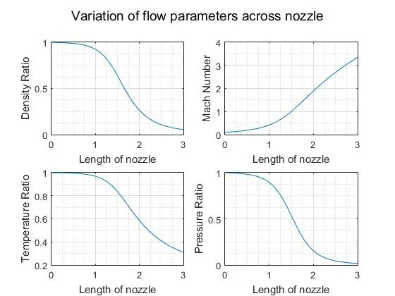
The variation in the non-dimensionalized flow field variables are plotted with respect to the length of the nozzle in non-conservative form.
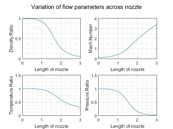
The variation in the non-dimensionalized flow field variables are plotted with respect to the length of the nozzle in conservative form.
b. Steady-state distribution of primitive variables inside the nozzle:
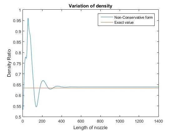
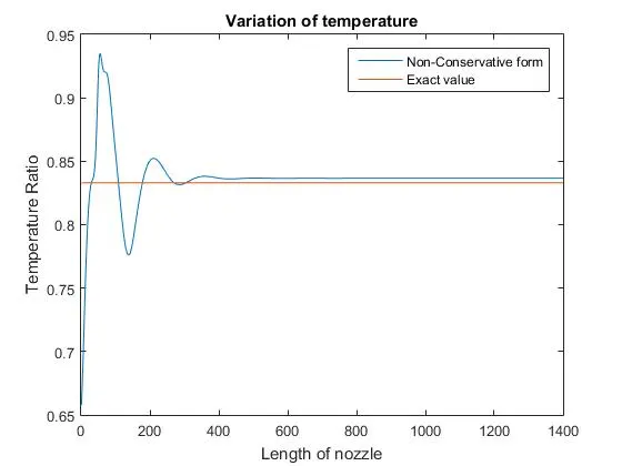
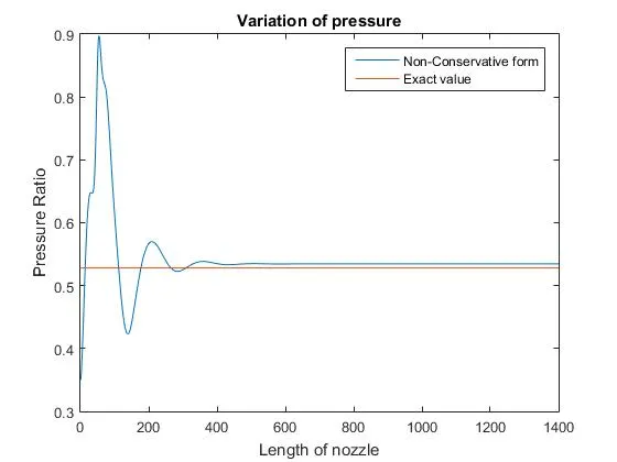
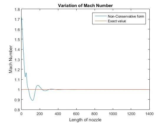
The throat is the section of minimum area, and is the section of interest when performing the study of convergence of the flow field variables at this section across the number of time steps.
Non-conservative form:
Conservative form:
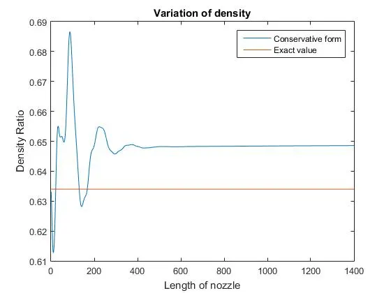
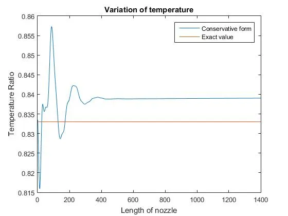
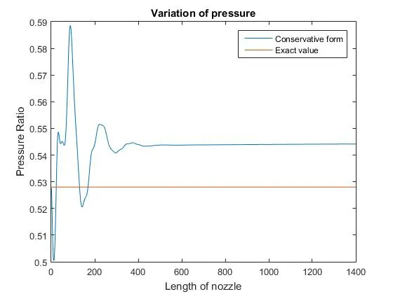
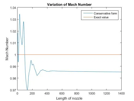
1. At early times, the time derivatives are large and they oscillate in value. These oscillations are related to the various unsteady compression and expansion waves which propagate through the nozzle during the transient process.
2. Later, the time derivatives rapidly grow small by six orders of magnitude over a span of 1000 time steps. Theoretically, the time derivatives should go to zero, which is impossible in a numerical scheme over a finite number of time steps. For all practical purposes, the numerical solution has arrived at a steady state solution.
3. The conservation form has a much lesser oscillation, while the non-conservation form does a much better job converging to the exact value of the analytical solution.
c. Variation of mass flow rate distribution inside the nozzle at different time steps during the time-marching process:
The mass flow rate varies with each time step until it settles to a constant steady state value.
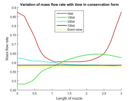
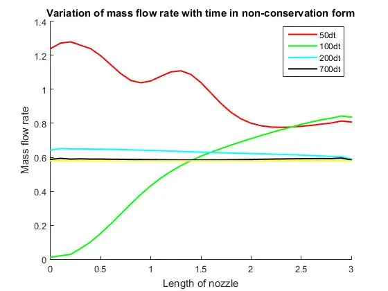
After 700 time steps, the mass flow rate is nearly constant throughout the nozzle for both forms of the governing equations.
d. Comparison of steady state mass flow rate across the nozzle: 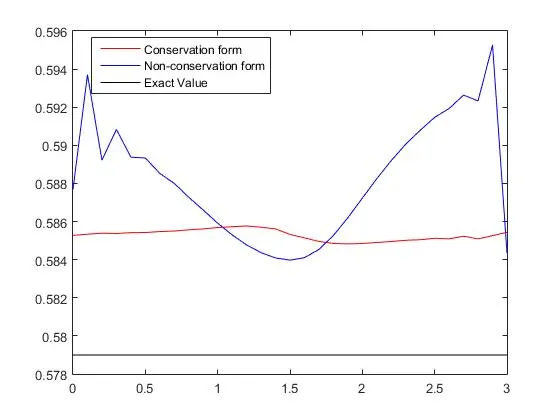
1. The conservation form gives a distribution that is much closer to being a constant. In contrast, the non-conservation results have(on the magnified scale) a sizeable variation with oscillations at both inflow and outflow boundaries. These variations are not apparent on a practical basis.
2. The steady-state mass flow results obtained with the conservation form are much closer to the exact analytical solution of p'A'V' = 0.579.
e. Grid dependence test:
The number of grid points is varied and the results are checked against the exact solution. The values are shows for the grid point capturing the throat section. For 61 grid points, the time step value is taken to be dt=0.01 so as to have a stable solution.
| Density Ratio | Temperature Ratio | Pressure Ratio | Mach Number | Mass Flow Rate | |
| Exact Analytical Solution | 0.634 | 0.833 | 0.528 | 1 | 0.579 |
| Non-conservative form(31 grid points) | 0.639 | 0.836 | 0.534 | 0.999 | 0.584 |
| Conservative form(31 grid points) | 0.648 | 0.839 | 0.544 | 0.987 | 0.585 |
| Non-conservative form(61 grid points) | 0.637 | 0.835 | 0.532 | 0.998 | 0.582 |
| Conservative form(61 grid points) | 0.639 | 0.835 | 0.534 | 0.997 | 0.582 |
1. For the samenumber of grid points, the non conservative form yields more accurate results than the conservative form.
2. Accuracy of the solution increases with an increase in number of grid points.
3. Solving the conservative form is more difficult as it involves more mathematical complexity.
4. The non-conservation form leads to better residuals.
5. There is no relative superiority between the forms of equations. The non-conservation form produces a better result for the primitive variables,while the conservation form produces more accurate results for the flux variables.