Week 3 - Taylor table method and Matlab code

Objective: 1. To derive 4th order approximations of the second-order derivative using

• Central differencing method
• Skewed right-sided difference
• Skewed left-sided difference

2. To write a program in Matlab to evaluate the second-order derivative of the analytical function exp(x)*cos(x) and compare it with the 3 numerical approximations derived along with the forward and backward difference scheems.

Derivation of the 4th order approximation of the second order derivative

Central Difference Scheme:

``(del^2f)/(delx^2) = (af(i-2) + bf(i-1) + cf(i) + df(i+1) + ef(i+2))/(Deltax^2)``

Terms	f(i)	`Deltaxf'(i)`	`Deltax^2f''(i)`	`Deltax^3f'''(i)``Deltax^4f''''(i)`	`Deltax^5f'''''(i)`
af(i-2)	a	-2a	4a/2	-8a/6	-16a/24
bf(i-1)	b	-b	b/2	-b/6	b/24
cf(i)	c	0	0	0	0
df(i+1)	d	d	d/2	d/6	d/24
ef(i+2)	e	2e	4e/2	8e/6	16e/24
af(i-2)+ bf(i-1) + cf(i) + df(i+1) + ef(i+2)	0	0	1	0	0

For the second order derivative, no other term except the second order derivative should be staying, hence all the other terms are equated to zero and the coefficient of the second order derivative is equated to 1.

Code:

function error = central_diff(x,dx)
% exp(x)*sin(x)
analytical_deriv = -(2*exp(x)*sin(x));

f = @(x) exp(x)*cos(x);
A = [1 1 1 1 1; 
    -2 -1 0 1 2;
    2 1/2 0 1/2 2;
    -8/6 -1/6 0 1/6 8/6;
    16/24 1/24 0 1/24 16/24];
B = [0; 0; 1; 0; 0];

C = linsolve(A,B);
a = C(1);
b = C(2);
c = C(3);
d = C(4);
e = C(5);

numerical_deriv = (a*f(x-2*dx) + b*f(x-dx) + c*f(x) + d*f(x+dx) + e*f(x+2*dx))/(dx^2);
    
error = abs(analytical_deriv - numerical_deriv);
end

Skewed Right Sided Scheme:

`(del^2f)/(delx^2) = (af(i) + bf(i+1) + cf(i+2) + df(i+3) + ef(i+4) + gf(i+5))/(Deltax^2)`

Terms	f(i)	`Deltaxf'(i)`	`Deltax^2f''(i)`	`Deltax^3f'''(i)``Deltax^4f''''(i)`	`Deltax^5f'''''(i)`	`Deltax^6f''''''(i)`
af(i)	a	-0	0	0	0	0
bf(i+1)	b	b/2	b/2	b/6	b/24	b/120
cf(i+2)	c	2c	4c/2	8c/6	16c/24	32c/120
df(i+3)	d	3d	9d/2	27d/6	81d/24	243d/120
ef(i+4)	e	4e	16e/2	64e/6	256e/24	1024e/120
gf(i+5)	5g	25g/2	125g/2	625g/24	3125g/120
af(i)+ bf(i+1) + cf(i+2) + df(i+3) + ef(i+4) + gf(i+5)	0	0	1	0	0	0

Code:

function error = right_skew_diff(x,dx)
% exp(x)*sin(x)
analytical_deriv = -(2*exp(x)*sin(x));

f = @(x) exp(x)*cos(x);
A = [1 1 1 1 1 1; 
    0 1 2 3 4 5;
    0 1/2 2 9/2 16/2 25/2;
    0 1/6 8/6 27/6 64/6 125/6;
    0 1/24 16/24 81/24 256/24 625/24;
    0 1/120 32/120 243/120 1024/120 3125/120];
    
      
B = [0; 0; 1; 0; 0; 0];

C = linsolve(A,B);
a = C(1);
b = C(2);
c = C(3);
d = C(4);
e = C(5);
g = C(6)
numerical_deriv = (a*f(x) + b*f(x+dx) + c*f(x+2*dx) + d*f(x+3*dx) + e*f(x+4*dx) + g*f(x+5*dx))/(dx^2);
    
error = abs(analytical_deriv - numerical_deriv);
end

Skewed Left Sided Scheme:

`(del^2f)/(delx^2) = (gf(i-5) + af(i-4) + bf(i-3) + cf(i-2) + df(i-1) + ef(i))/(Deltax^2)`

Terms	f(i)	`Deltaxf'(i)`	`Deltax^2f''(i)`	`Deltax^3f'''(i)``Deltax^4f''''(i)`	`Deltax^5f'''''(i)`	`Deltax^6f''''''(i)`
gf(i-5)	g	-5g	25g/2	-125g/6	625g/24	3125g/120
af(i-4)	a	-4a	8a	-64a/6	256a/24	1024a/120
bf(i-3)	c	-3b	9b/2	-27b/6	81b/24	243b/120
cf(i-2)	d	-2c	2c	-8c/6	16c/24	32c/120
df(i-1)	e	-d	d/2	-d/6	d/24	d/120
ef(i)	e	0	0	0	0	0
af(i)+ bf(i+1) + cf(i+2) + df(i+3) + ef(i+4) + gf(i+5)	0	0	1	0	0	0

Code:

function error = left_skew_diff(x,dx)
% exp(x)*sin(x)
analytical_deriv = -(2*exp(x)*sin(x));

f = @(x) exp(x)*cos(x);
A = [1 1 1 1 1 1; 
    -5 -4 -3 -2 -1 0;
    25/2 8 9/2 2 1/2 0;
    -125/6 -64/6 -27/6 -8/6 -1/6 0;
    625/24 256/24 81/24 16/24 1/24 0;
    3125/120 1024/120 243/120 32/120 1/120 0];
      
B = [0; 0; 1; 0; 0; 0];

C = linsolve(A,B);
g = C(1);
a = C(2);
b = C(3);
c = C(4);
d = C(5);
e = C(6)
numerical_deriv = (g*f(x-5*dx) + a*f(x-4*dx) + b*f(x-3*dx) + c*f(x-2*dx) + d*f(x-dx) + e*f(x))/(dx^2);
    
error = abs(analytical_deriv - numerical_deriv);
end

Code for Forward Differencing scheme:

function error = forward_diff(x,dx)
analytical_deriv = -2*(exp(x)*sin(x));
f = @(x) exp(x)*cos(x);
numerical_deriv = (f(x+dx) - f(x))/dx
error = abs(analytical_deriv - numerical_deriv);
end

Code for Backward Differencing scheme:

function error = backward_diff(x,dx)
analytical_deriv = -2*(exp(x)*sin(x));
f = @(x) exp(x)*cos(x);
numerical_deriv = (f(x) - f(x-dx))/dx
error = abs(analytical_deriv - numerical_deriv);
end

Main Code for plots:

close all
clear all
clc 
x = pi/4;
dx = linspace(pi/40,pi/4000000,50);
for i =1:50
    error_central(i) = central_diff(x,dx(i));
    error_left_skew(i) = left_skew_diff(x,dx(i));
    error_right_skew(i) = right_skew_diff(x,dx(i));
    error_FD(i) = forward_diff(x,dx(i));
    error_BD(i) = backward_diff(x,dx(i));
end
loglog(dx,error_central,'r','LineWidth',2);
hold on
loglog(dx,error_left_skew,'b','LineWidth',2);
hold on
loglog(dx,error_right_skew,'g','LineWidth',2);
xlabel('Grid length');
ylabel('Error');
title({'Comparison between different schemes for a second order derivative';'of 4th order accuracy'});
legend('Central Difference','Left Skewed Difference','Right Skewed Difference','location','southwest');

figure(2) 
loglog(dx,error_FD,'m','DisplayName','Forward Difference','LineWidth',2);
hold on
loglog(dx,error_BD,'c','DisplayName','Backward Difference','LineWidth',2);
legend('Location','northwest');
ylabel('Error')
xlabel('Grid Length')
title({'Comparison between Forward Difference and';'Backward Difference schemes'});

Output:

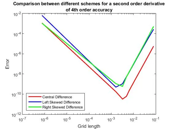
The errors from all the three differencing schemes have been calculated and stored in separate variables to be plotted. A loglog plot is used since the errors are incredibly small, and it would help to view the errors and compare them easily.

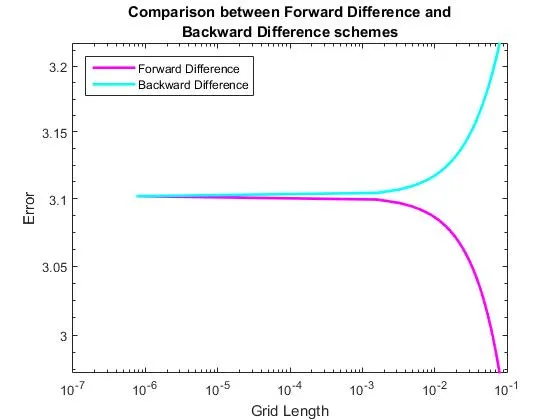
The forward and backward differences have also been calculated and their errors stored in seperate variables to be ready to be plotted.

Conclusion:

It is clearly seen that the fourth-order schemes are way more accurate than the first-order schemes namely, FDS and BDS. This happens since more terms from the Taylor series expansions are considered for the fourth-order approximation, than those for the first order approximation.

As for the 4th-order approximations, the central-differencing scheme proves to be more accurate than the skewed schemes. However, the skewed schemes are not completely redundant for that matter. In boundary nodes where cells on both sides are not available, skewed schemes play an important role. In CDS, information from both sides of the node is necessary, but that is not the case for skewed schemes.