Week 7 - Simulation of a 1D Super-sonic nozzle flow simulation using Macormack Method
Objective:- To simulate the isentropic flow through quasi 1D subsonic-supersonic nozzle by solving both the conservative and non-conservative forms of governing equations using the MacCormack's method and show
- Steady-state distribution of primitive variables inside the nozzle
- Time-wise variation of the primitive variables
- Variation of Mass flow rate distribution inside the nozzle at different time steps during the time- marching process
- Comparison of Normalized mass flow rate distributions of both forms
Given case:-
A nozzle is a device which converts the pressure energy of the fuid to the kinetic energy which results in the increase of the velocity of the flow.
1D quasi subsonic-supersonic nozzle means ,a nozzle with subsonic inlet(Mach<1) and supersonic outlet(Mach>1) with properties of the fluid flow varying only along the one dimension.
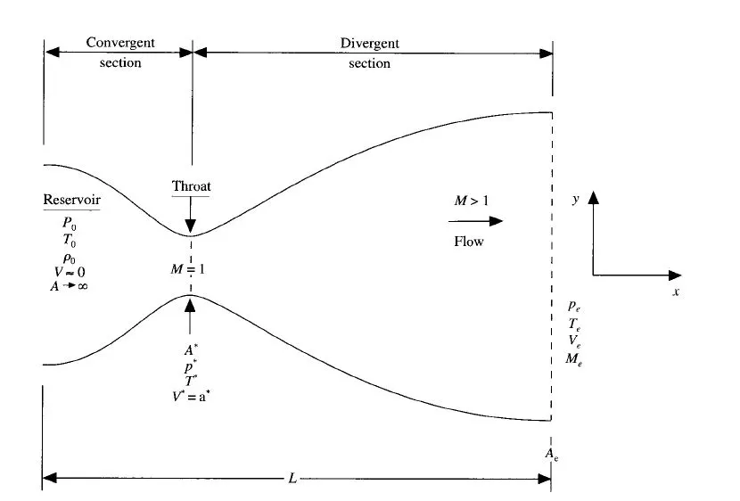
In the present case nozzle we have taken has 3-sections 1. Convergent section 2. Throat section and 3. Divergent section. Throat section has the mimimum area in the nozzle.We have assumed that the inlet of the nozzle is connected to the reservoir with temperature , pressure , density asT0 ,P0,`rho0`and at the inlet the velocity is approximated to zero.
Conservation vs Non-conservation form:-
To get the governing equations of the fluid flow a finite control volume is considered in region of the fluid flow.
If the the control volume is fixed in the space the governing equations obtained will be in the conservation from .
If the control volume is moving along the fluid flow then the equations obtained are called non-conservation form of governing equations
Governing equations
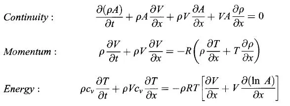
1.Non_conservation form:-
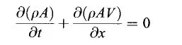
2.Conservation form:-
Continuity :
Momentum :

Energy :

where A= area of cross section (m^2) , p= pressure(pas) , V= velocity of flow(m/s)
T= temperature (k) , e= internal energy (J) , `rho`= density (kg/m^3) , t=time(sec)
Before solving the above equations we have to convert them into dimensionless form .Generally non-dimensionising is done to reduce the complexity of the equation.
let T0,`rho0`,V0 are the temperature,density and velocity at inlet.
Non-dimensional form of the variables
Temperature:- T'=T/T0;
Density:- `rho'`=`rho`/`rho0`
Velocity:- V'= V/a0
a0=speed of sound=sqrt(gamma*R*T0)
where R=gas constant
Area:- A'=A/A* A*=throat area
Time:- t'=t/(L/a0) L=length of the nozzle
Length:- x'=x/L
Mach number:-It is alredy a dimensionless number but, by writing it in the terms of the dimensionless variables we have
M = V'/sqrt(T')
By replacing the variables with their respective non dimensional forms the result we get is
Non-Conservative form:-
1.Countinuity equation:-

2.Momentum equation:-

3.Energy equation:-

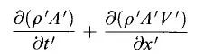
Conservative form:-
1.countinuity equation:-

2.Momentum equation:-

3.Energy equation:-

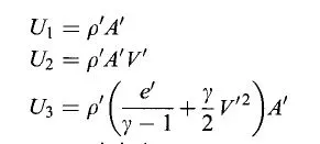
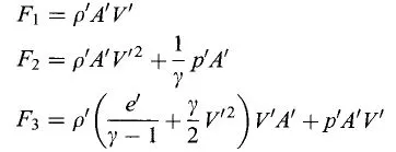
The above governing equations look complex and difficult to solve so it is expressed in terms of
Solution vector:-
Flux vector:-
Source term:-
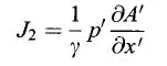
The conservative form of the governing equations written using solutio vector, flux vector and source term is
Countinuity equation:- ∂U1/∂t ‘ = -∂F1/∂x’
Momentum equation:- ∂U2/∂t ‘ = -∂F2/∂x’ + J2
Energy equation:- ∂U3/∂t ‘ = -∂F3/∂x’
MacCromack's method:-
It is a explicit finite differencing technique for solving the fluid flow .The main advantage of MacCormack's method is , we can get a second order accurate solutions without using the second order derivatives in the equation .It is easy to understand and program.
This method consits of 3 steps
1.Predictor step
2.Solution update
3.Corrector step
4.Taking Average
let us consider a equation du/dt=df/dx and values of 'f' is known at all places at time 't'
In predictor step the spatial derivative df/dx at time 't' is replacedn with forward differencing
( du/dt )t= f(i+1)-f(i)/dx;
and u(t+dt)=u(t)+ ( du/dt )t;
Now the solution obtained is only a predicted value of 'u' and it is only first order accurate.Using the values of 'u(t+dt)' values of 'f(t+dt)' is calculated and updated.
The values of the 'f' has to be update with the values obtained from the predictor step and then proceed to corrector step
In corrector step the spatial derivative is replaced with the backward differencing
(du/dt)t+dt=f(i)-f(i+1)/dx
After that mean of the du/dt from predictor and corrector step is calculated and stored in du/dt(avg).
Now this average value is taken and used to obtaine the final result.
u(t+dt)=u(t)+du/dt(avg)
The solution obtained now will be of the second order accurate.
Time step calculations:-
As we are using the explicit finite differencing technique the value of the time step 'dt' has to be decided as the solution becomes unstable for larger time steps .
dt=C*(dx/(A+V))
where C- courant number , dx-grid spacing , A-speed of sound , V-velocity of the flow
According to the stability criteria ,the Courant number must be less than '1' i.e., CFL<1 to keep the numerical solution to be stable.
The vaues of 'A' and 'V' along the x-direction .So , we get different values of 'dt'at each node.We have to consider the mimiumum value among them
dt=minimum(dt1,dt2,...........,dtn);
Solving
To solve the above case in both conservative and non conservative forms a function is written for both forms.
Before that we need initial conditions to define the present state of the system. As the partial differential equation we got are of hyperbolic in nature the solution can only be obtained by time marching.
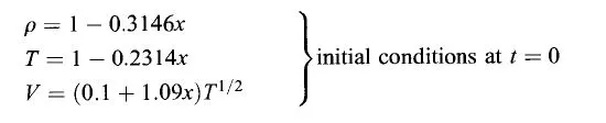
Initial conditions:-
Non-Conservative form:-
As the density ratio `rho'`=`rho`/`rho0` and T'=T/T0; at inlet `rho'`=1 , T'=1
and
Conservative form:-
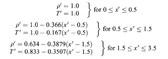
velocity- v=0.59/(`rho'`*a)
Non-Conservative form:-
Function:-
clear all
close all
clc
function [rho,T,v,p,M,m,rho_th,T_th,p_th,M_th]=Nonconserved(n,x,dx,a,gamma,C,th,nt)
% MacCorvack method

% initial conditions
rho=1-0.3146.*x;
T=1-0.2314.*x;
v=(0.1+(1.09.*x)).*T.^0.5;
p=rho.*T;

% mach number
   M=v./T.^0.5;
   M_initial=M;
%time step

dt=C*dx./(T.^0.5+v)
dt=min(dt)


% time loop
for k=1:nt

  rho_old=rho;
  v_old=v;
  T_old=T;


  % predictor method
  for j=2:n-1

    dv_dx=(v(j+1)-v(j))/dx;
    dlna_dx=(log(a(j+1))-log(a(j)))/dx;
    drho_dx=(rho(j+1)-rho(j))/dx;
    dT_dx=(T(j+1)-T(j))/dx;
    % countinity
    drho_dt_p(j)=-rho(j)*dv_dx-rho(j)*v(j)*dlna_dx-v(j)*drho_dx;
    % momentum equation
    dv_dt_p(j)=-v(j)*dv_dx-(1/gamma)*(dT_dx+((T(j)/rho(j))*drho_dx));
    % energy equation
    dT_dt_p(j)=-v(j)*dT_dx-(gamma-1)*T(j)*(dv_dx+(v(j)*dlna_dx));

    % solution update
    rho(j)=rho(j)+drho_dt_p(j)*dt;
    v(j)=v(j)+dv_dt_p(j)*dt;
    T(j)=T(j)+dT_dt_p(j)*dt;

  endfor

  % corrector method
  for j=2:n-1

    dv_dx=(v(j)-v(j-1))/dx;
    dlna_dx=(log(a(j))-log(a(j-1)))/dx;
    drho_dx=(rho(j)-rho(j-1))/dx;
    dT_dx=(T(j)-T(j-1))/dx;
    % countinity
    drho_dt_c(j)=-rho(j)*dv_dx-rho(j)*v(j)*dlna_dx-v(j)*drho_dx;
    % momentum equation
    dv_dt_c(j)=-v(j)*dv_dx-(1/gamma)*(dT_dx+((T(j)/rho(j))*drho_dx));
    % energy equation
    dT_dt_c(j)=-v(j)*dT_dx-(gamma-1)*T(j)*(dv_dx+(v(j)*dlna_dx));

  endfor

  % average values
  drho_dt=0.5.*(drho_dt_p+drho_dt_c);
  dv_dt=0.5.*(dv_dt_p+dv_dt_c);
  dT_dt=0.5.*(dT_dt_p+dT_dt_c);

  % final solution
  for i=2:n-1
   rho(i)=rho_old(i)+drho_dt(i)*dt;
   v(i)=v_old(i)+dv_dt(i)*dt;
   T(i)=T_old(i)+dT_dt(i)*dt;
  endfor

  % apply boundary conditions
  % inlet
  v(1)=2*v(2)-v(3);

  % outlet
  rho(n)=2*rho(n-1)-rho(n-2);
  v(n)=2*v(n-1)-v(n-2);
  T(n)=2*T(n-1)-T(n-2);

  p=rho.*T;
  % mach number
  M=v./T.^0.5;
  % mass flow rate
  m=rho.*a.*v;
  % value of the primitive variables at throat
  rho_th(k)=rho(th);
  T_th(k)=T(th);
  p_th(k)=p(th);
  M_th(k)=M(th);

  % plotting
  figure(1)
  if k==50
    plot(x,m,'r','linewidth',2)
    hold on
  elseif k==100
    plot(x,m,'b','linewidth',2)
    hold on
  elseif k==200
    plot(x,m,'y','linewidth',2)
    hold on
  elseif k==400
    plot(x,m,'g','linewidth',2)
    hold on
  elseif k==800
    plot(x,m,'k','linewidth',2)
    hold on
  elseif k==1000
    plot(x,m,'c','linewidth',2)
    hold on
   end

endfor
 title('variation of mass flow rate at different time steps')
 xlabel('non dimensional length')
 ylabel('non dimensional mass flow rate')
 legend('50','100','200','400','800','1000')
 grid on
endfunction
Conservative form:-
Function:-
% solving  consrevative form of equations
function [rho_c,T_c,v_c,p_c,M_c,rho_c_th,T_c_th,p_c_th,M_c_th,m_c]=conserved(n,x,dx,gamma,a,C,th,nt)
% MacCrovak methods

% initial conditions

for i=1:n
  if x(i)>=0 & x(i)<=0.5
    rho_c(i)=1;
    T_c(i)=1;
  elseif x(i)>=0.5 & x(i)<=1.5
    rho_c(i)=1-0.366*(x(i)-0.5);
    T_c(i)=1-0.167*(x(i)-0.5);
  elseif x(i)>=1.5 & x(i)<=3
    rho_c(i)=0.634-0.3879*(x(i)-1.5);
    T_c(i)=0.833-0.3507*(x(i)-1.5);
  end
end


% velocity ratio
v_c=0.59./(rho_c.*a);
% non dimensional pressure
p_c=rho_c.*T_c;
% mach number
M_c=v_c./T_c.^0.5;

% solution vector
u1=rho_c.*a;
u2=u1.*v_c;
u3=u1.*((T_c./(gamma-1))+((gamma/2).*(v_c.^2)));
m_c=u2;

u1_initial=u1;
u2_initial=u2;
u3_initial=u3;

%  time step
dt=min(C.*dx./((T_c.^0.5)+v_c));

% time loop
for k=1:nt

  u1_old=u1;
  u2_old=u2;
  u3_old=u3;

  % flux vector
   f1=u2;
   f2=(u2.^2./u1)+((gamma-1)/gamma).*(u3-((gamma/2).*u2.^2./u1));
   f3=((gamma.*u2.*u3)./u1)-((gamma*(gamma-1)/2).*(u2.^3./u1.^2));


  % predictor method
  for j=2:n-1
    df1_dx=(f1(j+1)-f1(j))/dx;
    df2_dx=(f2(j+1)-f2(j))/dx;
    df3_dx=(f3(j+1)-f3(j))/dx;
    dlna_dx=(log(a(j+1))-log(a(j)))/dx;
    j2(j)=((gamma-1)/gamma)*(u3(j)-((gamma*u2(j)^2)/(2*u1(j))))*dlna_dx;

    % countinuity equation
    du1_dt_p(j)=-df1_dx;
    % momentum equation
    du2_dt_p(j)=-df2_dx+j2(j);
    % energy equation
    du3_dt_p(j)=-df3_dx;
    % solution update
    u1(j)=u1_old(j)+du1_dt_p(j)*dt;
    u2(j)=u2_old(j)+du2_dt_p(j)*dt;
    u3(j)=u3_old(j)+du3_dt_p(j)*dt;

  end
   % solution update
     v_c=u2./u1;
     rho_c=u1./a;
     T_c=(gamma-1).*((u3./u1)-((gamma/2).*v_c.^2));
     p_c=rho_c.*T_c;

    % flux vector
    f1=u2;
    f2=(u2.^2./u1)+((gamma-1)/gamma).*(u3-((gamma/2).*u2.^2./u1));
    f3=((gamma.*u2.*u3)./u1)-((gamma*(gamma-1)/2).*(u2.^3./u1.^2));

  % corrector method
  for j=2:n-1

   df1_dx_c=(f1(j)-f1(j-1))/dx;
   df2_dx_c=(f2(j)-f2(j-1))/dx;
   df3_dx_c=(f3(j)-f3(j-1))/dx;
   dlna_dx_c=(log(a(j))-log(a(j-1)))/dx;
   j2_c(j)=((gamma-1)/gamma)*(u3(j)-((gamma*u2(j)^2)/(2*u1(j))))*dlna_dx_c;

   % countinuity equations
   du1_dt_c(j)=-df1_dx_c;
   % momentum equation
   du2_dt_c(j)=-df2_dx_c+j2_c(j);
   % energy equation
   du3_dt_c(j)=-df3_dx_c;

  end

  % average value
  du1_dt=0.5.*(du1_dt_p+du1_dt_c);
  du2_dt=0.5.*(du2_dt_p+du2_dt_c);
  du3_dt=0.5.*(du3_dt_p+du3_dt_c);

  for i=2:n-1
    u1(i)=u1_old(i)+du1_dt(i)*dt;
    u2(i)=u2_old(i)+du2_dt(i)*dt;
    u3(i)=u3_old(i)+du3_dt(i)*dt;
  end
  % inlet
   u2(1)=2*u2(2)-u2(3);

  % outlet
  u1(n)=2*u1(n-1)-u1(n-2);
  u2(n)=2*u2(n-1)-u2(n-2);
  u3(n)=2*u3(n-1)-u3(n-2);

  % decoding of variables
  m_c=u2;
  v_c=u2./u1;
  rho_c=u1./a;
  T_c=(gamma-1).*((u3./u1)-((gamma/2).*v_c.^2));
  p_c=rho_c.*T_c;
  M_c=v_c./T_c.^0.5;

  % value of the primitive variables at throat
  rho_c_th(k)=rho_c(th);
  T_c_th(k)=T_c(th);
  p_c_th(k)=p_c(th);
  M_c_th(k)=M_c(th);

  % plotting
  figure(2)
  if k==50
    plot(x,m_c,'r','linewidth',2)
    hold on
  elseif k==100
    plot(x,m_c,'b','linewidth',2)
    hold on
  elseif k==200
    plot(x,m_c,'y','linewidth',2)
    hold on
  elseif k==400
    plot(x,m_c,'g','linewidth',2)
    hold on
  elseif k==800
    plot(x,m_c,'k','linewidth',2)
    hold on
  elseif k==1000
    plot(x,m_c,'c','linewidth',2)
    hold on
   end

endfor
  title('variation of mass flow rate at different time steps')
  xlabel('non dimensional length')
  ylabel('non dimensional mass flow rate')
  legend('50','100','200','400','800','1000')
  grid on
endfunction
In both of the functions inputs needed are same ,they are defined as follows
n=31
x=discretization of length of nozzle into n grid points
dx=grid spacing
nt=no of time steps
C=courant number
dt=time step length
After the functions are written and executed another program is written in a new script file in which inputs are defined and both the functions are called .
% inputs
n=61;
x=linspace(0,3,n);
dx=x(2)-x(1);
gamma=1.4;
% Area
a=1+2.2.*(x-1.5).^2;
% throat section position
th=(n-1)/2;
% Courant number
C=0.5;
% no of time steps
nt=1000;
% time
t=1:nt;

% non conservation solution
[rho,T,v,p,M,m,rho_th,T_th,p_th,M_th]=Nonconserved(n,x,dx,a,gamma,C,th,nt)

% steady state distribution of primitive variables within nozzle
figure(3)
subplot(4,1,1)
plot(x,rho,'linewidth',2)
xlabel('x/L')
ylabel(' density ratio')
title('steady state distributation of variables')
grid on

subplot(4,1,2)
plot(x,T,'linewidth',2)
xlabel('x/L')
ylabel('T/T0')
grid on

subplot(4,1,3)
plot(x,p,'linewidth',2)
xlabel('x/L')
ylabel('p/p0')
grid on

subplot(4,1,4)
plot(x,M,'linewidth',2)
xlabel('x/L')
ylabel('M')
grid on


% time wise variation of primitive variables at throat section
figure(4)
subplot(4,1,1)
plot(t,rho_th,'linewidth',2)
xlabel('time steps')
ylabel('density ratio')
title('variation of variables w.r.t time steps')
grid on
axis([0 1000 0 1.5])

subplot(4,1,2)
plot(t,T_th,'linewidth',2)
xlabel('time steps')
ylabel('T/T0')
grid on
axis([0 1000 0 1.5])

subplot(4,1,3)
plot(t,p_th,'linewidth',2)
xlabel('time steps')
ylabel('p/p0')
grid on
axis([0 1000 0 1.5])

subplot(4,1,4)
plot(t,M_th,'linewidth',2)
xlabel('time steps')
ylabel('M')
grid on
axis([0 1000 0 1.5])

% conservative solutions
[rho_c,T_c,v_c,p_c,M_c,rho_c_th,T_c_th,p_c_th,M_c_th,m_c]=conserved(n,x,dx,gamma,a,C,th,nt)

% steady state distribution of variables within nozzle
figure(5)
subplot(4,1,1)
plot(x,rho_c,'linewidth',2)
xlabel('x/L')
ylabel(' density ratio')
title('steady state distributation of variables')
grid on

subplot(4,1,2)
plot(x,T_c,'linewidth',2)
xlabel('x/L')
ylabel('T/T0')
grid on

subplot(4,1,3)
plot(x,p_c,'linewidth',2)
xlabel('x/L')
ylabel('p/p0')
grid on

subplot(4,1,4)
plot(x,M_c,'linewidth',2)
xlabel('x/L')
ylabel('M')
grid on


% time wise variation of primitive variables at throat section
figure(6)
subplot(4,1,1)
plot(t,rho_c_th,'linewidth',2)
xlabel('time steps')
ylabel('density ratio')
title('variation of variables w.r.t time steps')
grid on
axis([0 1000 0.5 1])

subplot(4,1,2)
plot(t,T_c_th,'linewidth',2)
xlabel('time steps')
ylabel('T/T0')
grid on
axis([0 1000 0.5 1])

subplot(4,1,3)
plot(t,p_c_th,'linewidth',2)
xlabel('time steps')
ylabel('p/p0')
grid on
axis([0 1000 0.5 1])

subplot(4,1,4)
plot(t,M_c_th,'linewidth',2)
xlabel('time steps')
ylabel('M')
grid on
axis([0 1000 0.5 1])

% plotting mass flow rate
figure(7)
plot(x,m,'r','linewidth',2)
hold on
plot(x,m_c,'b','linewidth',2)
grid on
axis([ 0 3 0.56 0.6])
title('mass flow rate distributation')
legend('non conserves','conserved')
Upon executing the above program the plots and results we got is
Non-Conservative form:-
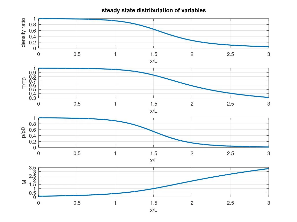
1.Steady state distribution of variables along the length of nozzle
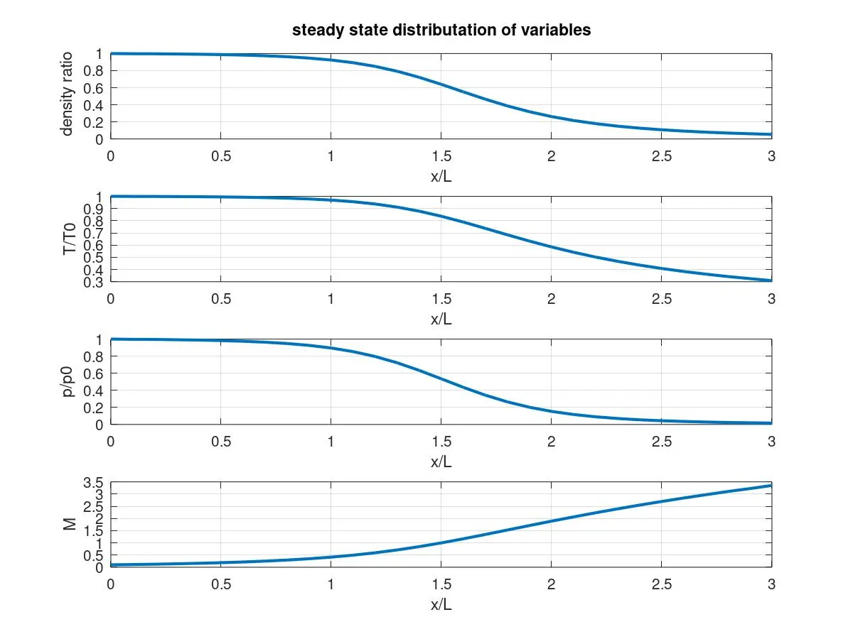
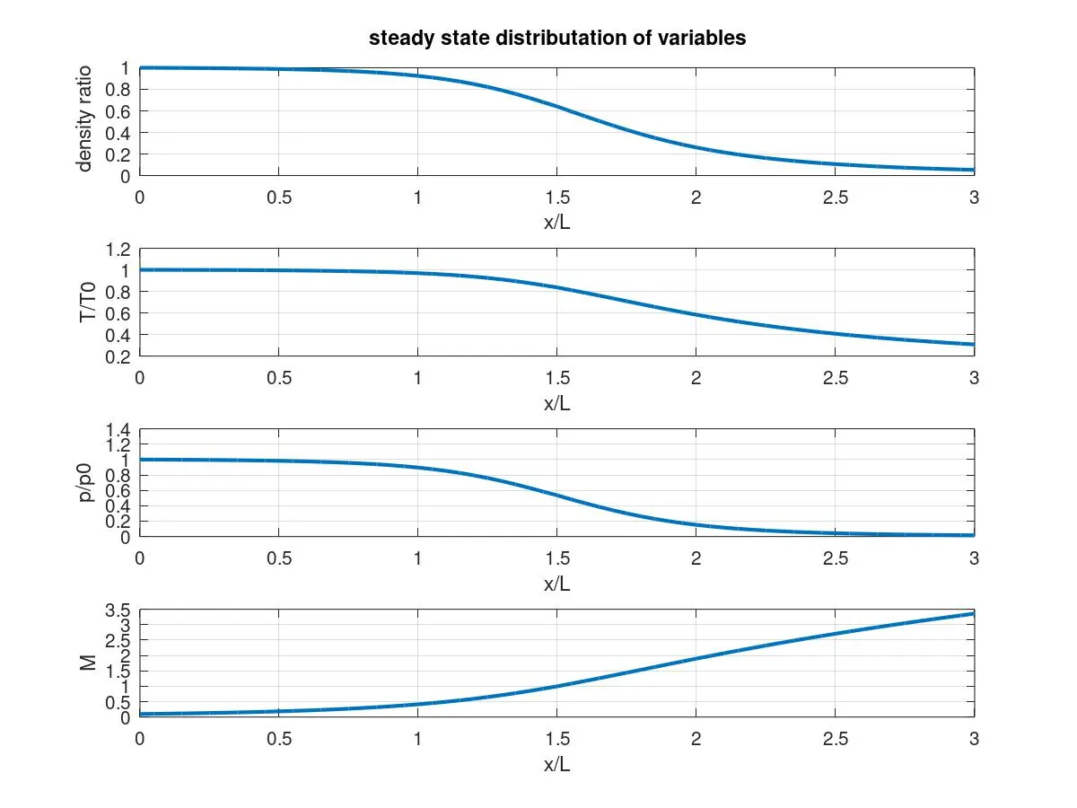
By observing the above results it is clear that the pressure is dropping as we procced along the nozzle and velocity is incresing.Which signifies that kinetatic energy of the flow is increased at the expense of the pressure energy.
By looking at mach no variation 'M' it says at intlet the flow is subsonic ,at outlet flow is super sonic as M=3.25 and sonic at throat section(x=1.5) M=1;
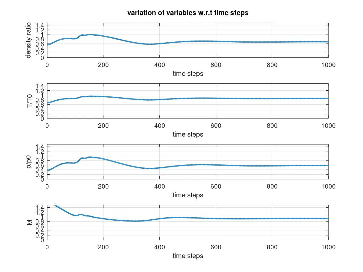
2.Time wise variation of primitive variables(at throat)
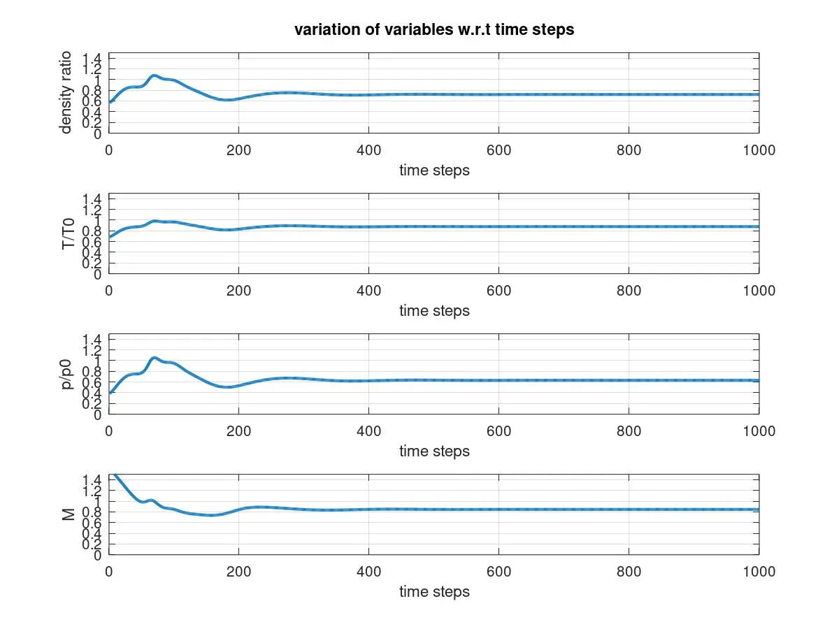
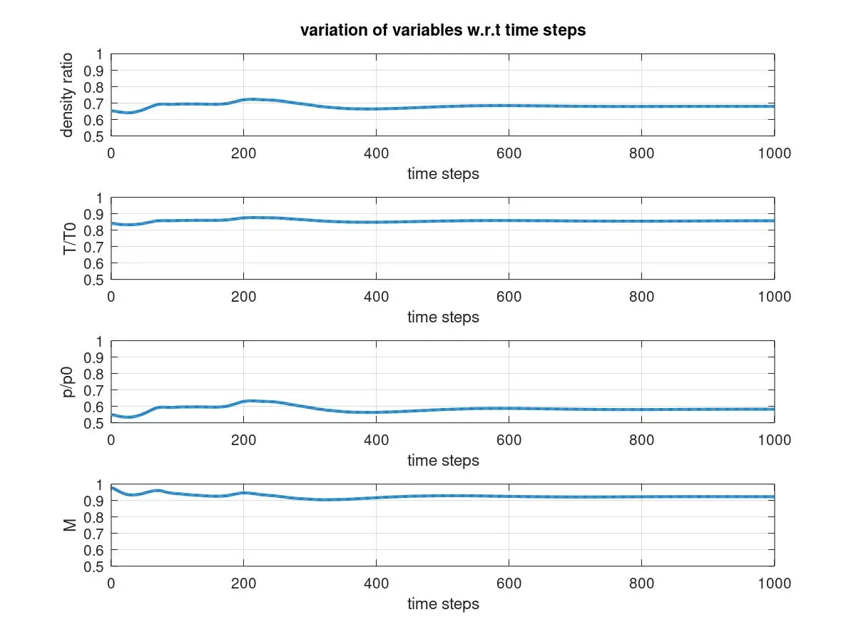
By observing the time wise variations of the variables we can say that upto 400-500 time steps the system is unsteady and beyond 600 time steps the system reached to the steady state i.e., no variation of the properties is observed .
In the present case we have used 1000 time steps , we can reduce the no of time steps to 650 to reduce the solution time .
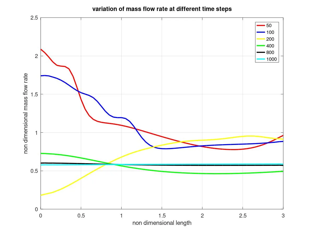
3.Mass flow rate distribution at various time steps:-
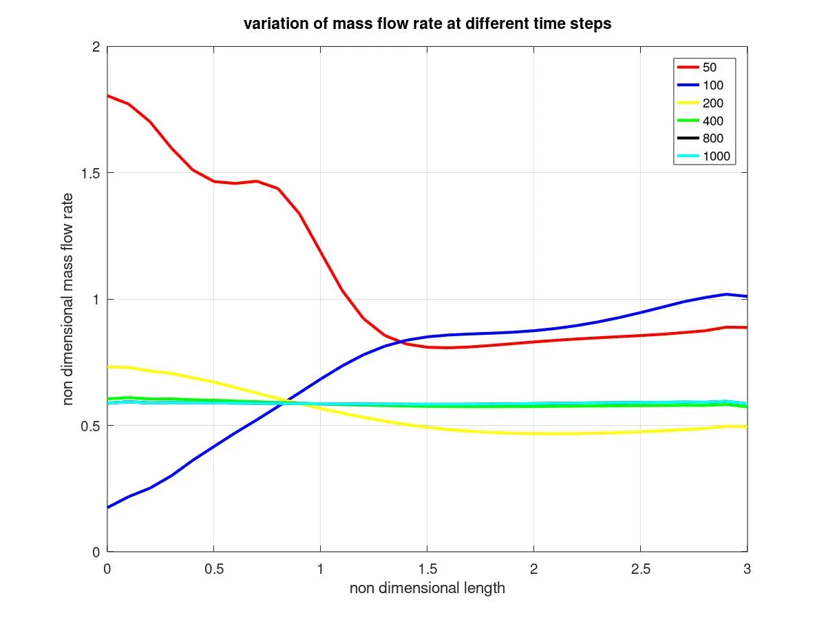
At amaller time steps i.e., at 50 , 100 , 200 the variation of mass flow rate along length is very high as we can see form the graph , but as the solution progress variation in the mass flow rate becomes negligble .At higher time steps of 800,1400 the mass flow rate became almost constant.
Conservative form:-
1.Steady state distribution of variables along the length of nozzle:-
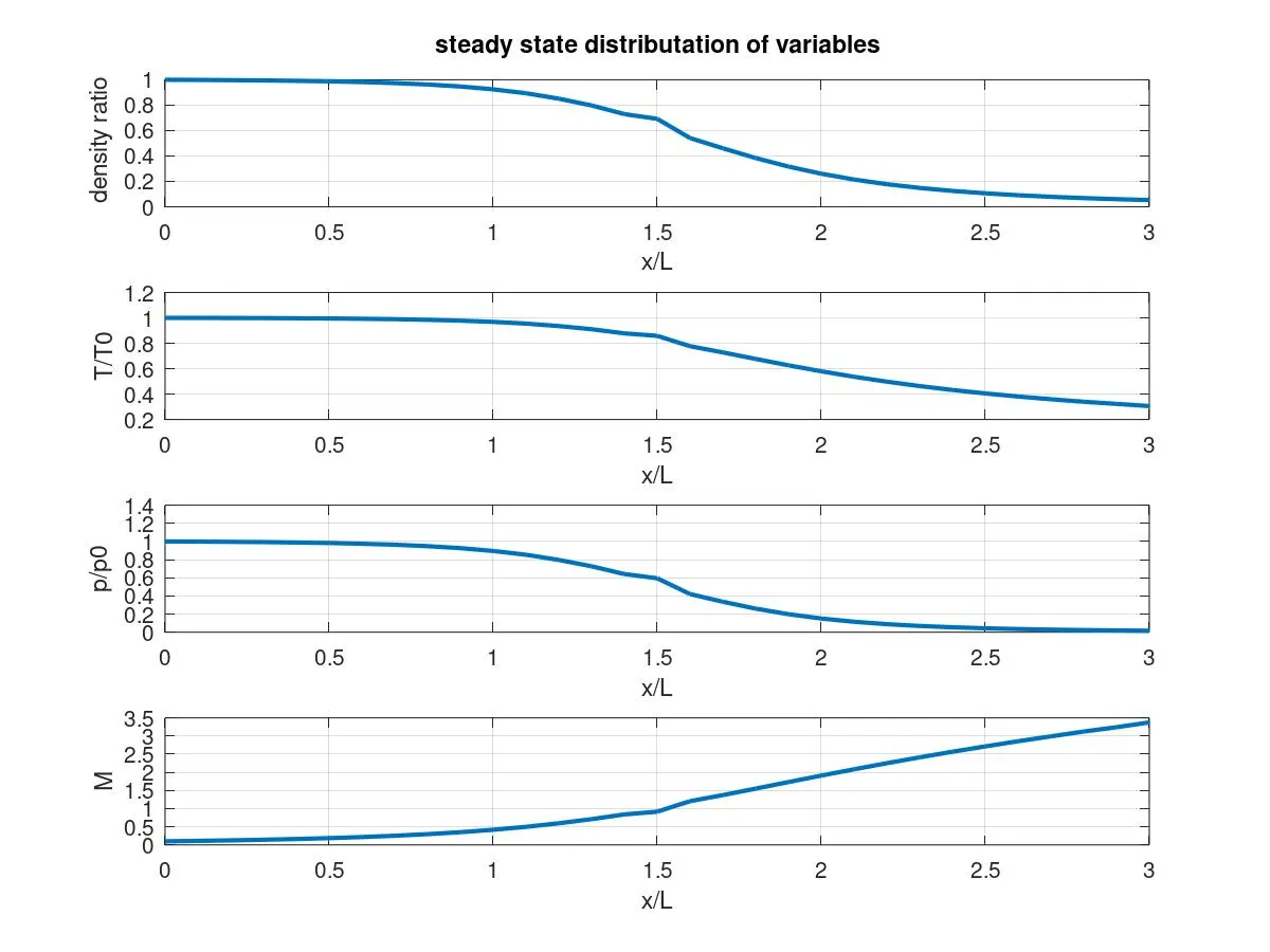
The steady state distribution of the primitive variables in non dimensional along the nozzle lenght is shown in the above graph.
Velocity of the flow is increased at the expense of the pressure.
2.Time wise variation of primitive variables(at throat):-
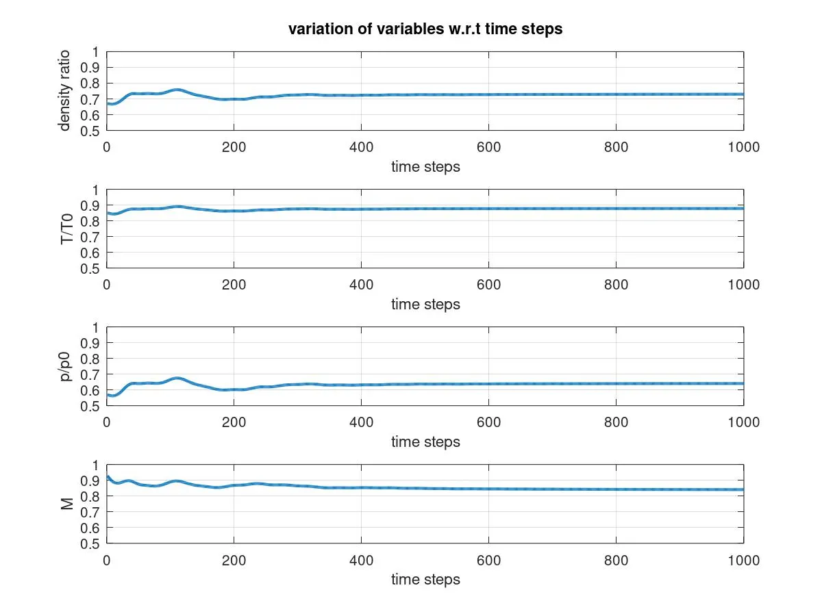
The time wise variation of the variables at throat section is shown .Compared to the non conservative form consrvative case has less deviation of the results .The steady state is reached at 600 time steps
3.Mass flow rate distribution at various time steps:-
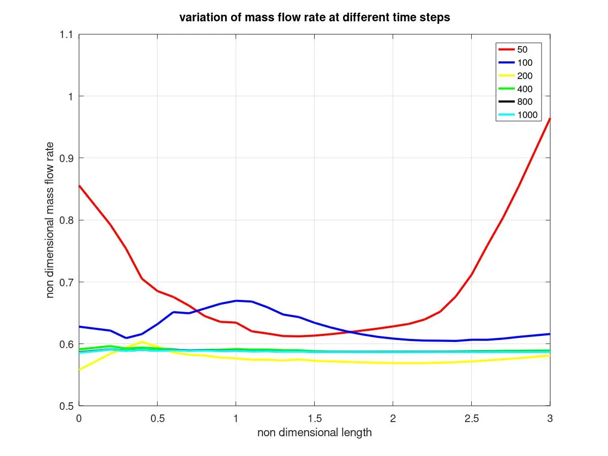
Mass flow rate at different time steps is observed .It is clear that at smaller time steps the variation of mass flow rate along nozzle is very high ,as the no of steps increases the deviation gradually reduces and becomes zero.
At time step 800 and greater no variation is obsereved the value is almost constant.
4.Mass flow rate (non conservative vs conservative form):-
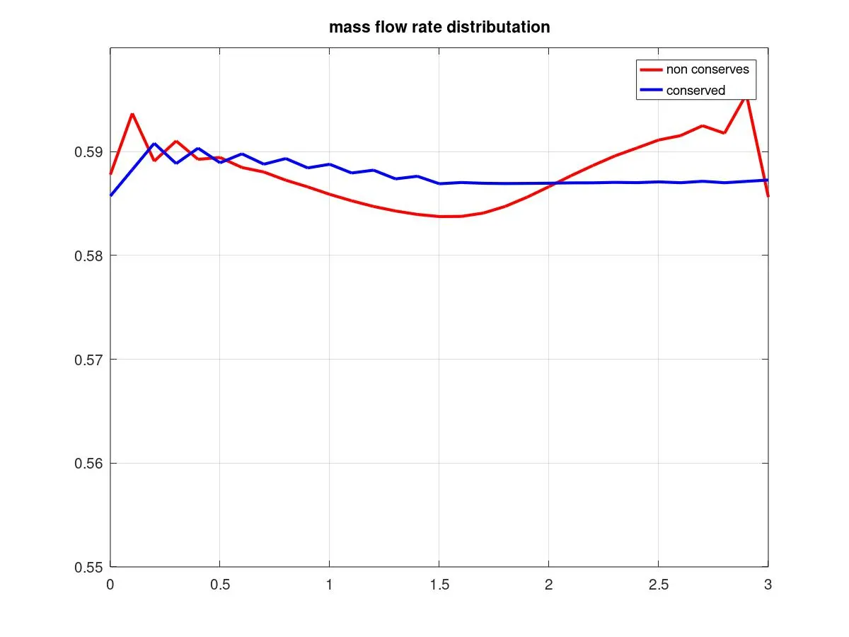
Above is the steady state mass flow rate distribution along the length of the nozzle .In case of conserved form the mass flow rate is more stable compared to the non conserved form i.e., the values of the mass flow rate obtained by conservation form are more accurate.
Grid independence test:-
It is performed by reducing the grid size and see weather the change in the grid size has any effect on the final solution or not.In the above case we have taken 31 grids .Now the analysis is done with 61 grids, which is a finer mesh than the previous one.
The results and plots obtained by changing the no of gride n= 61 is
Non conservation form
Conservative form:-
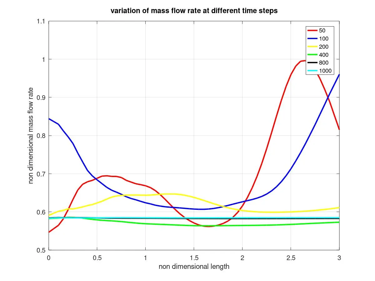
By observing the plots we can say that there is no change in the steady state solution in case of both coarse mesh(n=31) and fine mesh(n=61).
Though their is a small difference in the values at earlier time steps as the solution progress it vanished . The time step according to the stability criteria in this case is 0.01 so the solution has taken around 800 time steps to reach steady state.