Week 7 - Simulation of a 1D Super-sonic nozzle flow simulation using Macormack Method
% witting program for simulation of 1D NOZZEL SUPERSONIC FLO USING MACORMAC
% METHOD
clear all
close all
clc

%defing the inputs
%number of grids points
n=31;
x=linspace(0,3,n);
dx=x(2)-x(1);


gamma=1.4;

%numbers of time steps
nt=1400;
CFL=0.5;

%defing the function for non conservation form of simulation
tic;
[mass_flow_rate_nc, presure_nc, mach_num_nc, rho_nc, v_nc, T_nc, rho_trottle_nc, v_trottle_nc, T_trottle_nc, mass_flow_rate_trottle_nc, presure_trottle_nc, mach_num_trottle_nc]=non_conservative_form_original(x,dx,n,gamma,nt,CFL)
time_elapsed=toc;
fprintf('time elapesed for non coservation form:%f',time_elapsed)
hold on
%ploting the graphs
figure(3)
%for density
subplot(4,1,1)
plot(linspace(1,nt,1400),rho_trottle_nc,"Color","m");
ylabel("density")
legend({'density at trottle'})
title('timestep variation at trottle area-non conservation form')

%for tempreture
subplot(4,1,2)
plot(linspace(1,nt,1400),T_trottle_nc,"Color","b");
ylabel("tempreture")
legend({'tempreture at trottle'})
title('timestep variation at trottle area-non conservation form')

% for presure
subplot(4,1,3)
plot(linspace(1,nt,1400),presure_trottle_nc,"Color","r");
ylabel("presure")
legend({'presure at trottle'})
title('timestep variation at trottle area-non conservation form')

%for mach number
subplot(4,1,4)
plot(linspace(1,nt,1400),mach_num_trottle_nc,"Color","m");
xlabel('time step')
ylabel("mach nuber")
legend({'mach num at trottle'})
title('timestep variation at trottle area-non conservation form')


% steady sTATE simulation for primitive value for nom conservation form
figure(4)

%for density
subplot(4,1,1)
plot(x,rho_nc,"Color","m");
ylabel("density")
legend({'density'})
title('timestep variation at trottle area-non conservation form')

%for tempreture
subplot(4,1,2)
plot(x,T_nc,"Color","b");
ylabel("tempreture")
legend({'tempreture'})
title('timestep variation at trottle area-non conservation form')

% for presure
subplot(4,1,3)
plot(x,presure_nc,"Color","r");
ylabel("presure")
legend({'presure'})
title('timestep variation at trottle area-non conservation form')

%for mach number
subplot(4,1,4)
plot(x,rho_nc,"Color","m");
xlabel('nozzel lenth')
ylabel("mach nuber")
legend({'mach num at trottle'})
title('timestep variation at trottle area-non conservation form')

% %defing the function for conservation form of simulation
tic;
[mass_flow_rate_c, presure_c, mach_num_c, rho_c,v_c, T_c, rho_trottle_c, v_trottle_c, T_trottle_c, mass_flow_rate_trottle_c, presure_trottle_c, mach_num_trottle_c]=conservation_form(x,dx,n,gamma,nt,CFL);
time_elapsed_c=toc;
fprintf('time elapesed for coservation form:%f',time_elapsed_c)
hold on

%plotting
figure(5)
%for density
subplot(4,1,1)
plot(linspace(1,nt,1400),rho_trottle_c,'Color','m');
ylabel("density")
legend({'density at trottel'})
title('timestep variation at trottle area- conservation form')

%for tempreture
subplot(4,1,2)
plot(linspace(1,nt,1400),T_trottle_c,'Color',"b");
ylabel("tempreture")
legend({'tempreture at trottle'})
title('timestep variation at trottle area- conservation form')

% for presure
subplot(4,1,3)
plot(linspace(1,nt,1400),presure_trottle_c,"Color","r");
ylabel("presure")
legend({'presure at trottle'})
title('timestep variation at trottle area- conservation form')

%for mach number
subplot(4,1,4)
plot(linspace(1,nt,1400),mach_num_trottle_c,"Color","m");
xlabel('time step')
ylabel("mach nuber")
legend({'mach num at trottle'})
title('timestep variation at trottle area- conservation form')


% steady sTATE simulation for primitive value for nom conservation form
figure(6)

%for density
subplot(4,1,1)
plot(x,rho_c,"Color","m");
ylabel("density")
legend({'density'})
title('timestep variation at trottle area- conservation form')


%for tempreture
subplot(4,1,2)
plot(x,T_c,"Color","b");
ylabel("tempreture")
legend({'tempreture'})
title('timestep variation at trottle area-conservation form')

% for presure
subplot(4,1,3)
plot(x,presure_c,"Color","r");
ylabel("presure")
legend({'presure'})
title('timestep variation at trottle area- conservation form')

%for mach number
subplot(4,1,4)
plot(x,mach_num_c,"Color","m");
xlabel('nozzel lenth')
ylabel("mach nuber")
legend({'mach num at trottle'})
title('timestep variation at trottle area- conservation form')


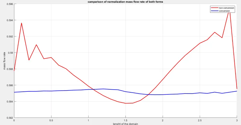
%camparing the plots of narmalization mass flow rte of both forms

figure(7)
hold on
plot(x,mass_flow_rate_nc,'r','linewidth',2)
hold on
plot(x,mass_flow_rate_c,'b','linewidth',2)
hold on
grid on
legend('non conversion','conversion')
xlabel('lenght of the domain')
ylabel('mass flow rate')
title('camparison of narmalization mass flow rate of both forms')
Function for consevation form:
%writting the function for non conservation form using macormac method
function [mass_flow_rate_c, presure_c, mach_num_c, rho_c, v_c, T_c, rho_trottle_c, v_trottle_c, T_trottle_c, mass_flow_rate_trottle_c, presure_trottle_c, mach_num_trottle_c]=conservation_form(x,dx,n,gamma,nt,CFL)
%[mass_flow_rate_c, presure_c, mach_num_c, rho_c, v_c, T_c, rho_trottle_c, v_trottle_c, T_trottle_c, mass_flow_rate_trottle_c, presure_trottle_c, mach_num_trottle_c]=conservation_form(x,dx,n,gamma,nt,CFL);
%defining the intial boundry condition for density and tempreture
for m =1:n
    if(x(m) >=0 && x(m) <=0.5)
        rho_c(m)=1;
        T_c(m) =1;
    elseif (x(m) >=0.5 && x(m) <=1.5)
        rho_c(m)=1-0.366*(x(m)-0.5);
        T_c(m) =1-0.167*(x(m)-0.5);
    elseif  (x(m) >=1.5 && x(m) <=3.5)
         rho_c(m)=0.634-0.3879*(x(m)-1.5);
        T_c(m) =0.833-0.3507*(x(m)-1.5);
    end
end

%defining for velocity
a=1+2.2*(x-1.5).^2;
v_c =0.59./(rho_c.*a);
presure_c=rho_c.*T_c;

% defining the trottle
trottle = find(a==1);

% defing the initiel solution variabels
U1 =rho_c.*a;
U2 =rho_c.*a.*v_c;
U3 =rho_c.*a.*(T_c./(gamma-1))+((gamma/2).*v_c.^2);

%defining the time loop


for k =1:nt

    %defining the time step

    dt =min(CFL.*dx./(sqrt(T_c)+v_c));

    %defing the old values
    U1_old=U1;
    U2_old=U2;
    U3_old=U3;

    %calculating the flux

    F1=U2;
    F2=((U2.^2)./U1)+((gamma-1)/gamma)*(U3-(gamma/2)*((U2.^2)./U1));
    F3=((gamma*U2.*U3)./U1)-(gamma*(gamma-1)*((U2.^3)./(2*U1.^2)));

    % calculatinf the predector method

    for j = 2:n-1

        % calculating the souse term
        J2(j)=(1/gamma)*rho_c(j)*T_c(j)*((a(j+1)-a(j))/dx);

        % continuty eqution

        dU1_dt_p(j)=-((F1(j+1)-F1(j))/dx);

        % momentum equation
         dU2_dt_p(j)=-((F2(j+1)-F2(j))/dx)+J2(j);


         %energy equation
          dU3_dt_p(j)=-((F3(j+1)-F3(j))/dx);

          % updating the soluton vector
          U1(j)=U1(j)+dU1_dt_p(j)*dt;
          U2(j)=U2(j)+dU2_dt_p(j)*dt;
          U3(j)=U3(j)+dU3_dt_p(j)*dt;
    end

    %updating the flux
    F1=U2;
    F2=((U2.^2)./U1)+((gamma-1)/gamma)*(U3-(gamma*0.5*(U2.^2)./U1));
    F3=((gamma*U2.*U3)./U1)-((gamma*0.5*(gamma-1)*(U2.^3)./(U1.^2)));


    % know calculating for currector method
    for j=2:n-1

% calculating the souse term
        J2(j)=(1/gamma)*rho_c(j)*T_c(j)*((a(j)-a(j-1))/dx);

        % continuty eqution

        dU1_dt_c(j)=-((F1(j)-F1(j-1))/dx);

        % momentum equation
         dU2_dt_c(j)=-((F2(j)-F2(j-1))/dx)+J2(j);


         %energy equation
          dU3_dt_c(j)=-((F3(j)-F3(j-1))/dx);

    end

    %computing the avarege value

    dU1_dt_av=0.5*(dU1_dt_p+dU1_dt_c);
    dU2_dt_av=0.5*(dU2_dt_p+dU2_dt_c);
    dU3_dt_av=0.5*(dU3_dt_p+dU3_dt_c);

    % calculating the final solution

    for m=2:n-1
        U1(m)=U1_old(m)+dU1_dt_av(m)*dt;
        U2(m)=U2_old(m)+dU2_dt_av(m)*dt;
        U3(m)=U3_old(m)+dU3_dt_av(m)*dt;
    end

    %appliying the boundry conditions
    % at inlets
    U1(1)=rho_c(1)*a(1);
    U2(1)=2*U2(2)-U2(3);
    v_c(1)=U2(1)./U1(1);
    U3(1)=U1(1)*((T_c(1)/(gamma-1))+((gamma/2)*(v_c(1)).^2));

    %at outlet
     U1(n)=2*U1(n-1)-U1(n-2);
     U2(n)=2*U2(n-1)-U2(n-2);
     U3(n)=2*U3(n-1)-U3(n-2);

     %final primitive value update
     rho_c=U1./a;
     v_c=U2./U1;
     T_c=(gamma-1)*((U3./U1)-(gamma/2)*(v_c).^2);

     % defing the mass flow rate

        %defing the flow rate
        mass_flow_rate_c = rho_c.*a.*v_c;
        presure_c = rho_c.*T_c;
        mach_num_c = (v_c./sqrt(T_c));

        % calculating the variables at trottle
        rho_trottle_c(k) = rho_c(trottle);
        T_trottle_c(k) = T_c(trottle);
        v_trottle_c(k) = v_c(trottle);
        mass_flow_rate_trottle_c(k) =  mass_flow_rate_c(trottle);
        presure_trottle_c(k) = presure_c(trottle);
        mach_num_trottle_c(k) = mach_num_c(trottle);

         %comparing the non dimensional mass flow at different time step
         %plotting
         figure(2);

        if  k == 50
             plot(x,mass_flow_rate_c,'b','linewidth',1)
             hold on

        elseif k == 150
              plot(x,mass_flow_rate_c,'c','linewidth',1)
          hold on

        elseif k == 200
             plot(x,mass_flow_rate_c,'k','linewidth',1)
          hold on

        elseif k == 400
             plot(x,mass_flow_rate_c,'g','linewidth',1)
           hold on

        elseif k == 800
             plot(x,mass_flow_rate_c,'m','linewidth',1)
             hold on
        end

end
%labeling
xlabel('domain')
ylabel('mass flow rate conservation')
title('camparing the non dimensinal mass flow rate at diffrent time steps-conservation form ')
legend({'50th time step','150th time step','200th time step','400th time step','800th time step'})
grid on
Function for non conservation form:
%writting the function for non conservation form using macormac method
function [mass_flow_rate_nc, presure_nc, mach_num_nc, rho_nc, v_nc, T_nc, rho_trottle_nc, v_trottle_nc, T_trottle_nc, mass_flow_rate_trottle_nc, presure_trottle_nc, mach_num_trottle_nc]=non_conservative_form_original(x,dx,n,gamma,nt,CFL)


%defining the intial boundry condition
rho_nc=1 - 0.3146*x;
T_nc =1 - 0.2341*x;
v_nc=(0.1+1.09*x).*T_nc.^0.5;

%area of the nozzel

a = 1+2.2*(x-1.5).^2;

% defing trottle
trottle = find(a==1);

%defing the time loop
%defing the nodes

for k =1:nt
    dt =min(CFL.*dx./(sqrt(T_nc)+v_nc));

    %defing the old values

    rho_old=rho_nc;
    T_old=T_nc;
    v_old =v_nc;

    %know we have to solve  for pridictor method

    for j =2:n-1


        % simplifying the speciel terms there fore we have equation for continity momentum energy in that equation we are descritizing using forword scheme
        dv_dx =(v_nc(j+1)-v_nc(j))./dx;
        drho_dx =(rho_nc(j+1)-rho_nc(j))./dx;
        dT_dx =(T_nc(j+1)-T_nc(j))./dx;
        dlog_a_dx =(log(a(j+1))-log(a(j)))./dx;

        % continuty equation
        drho_dt_p(j)=-rho_nc(j)*dv_dx-rho_nc(j)*v_nc(j)*dlog_a_dx-v_nc(j)*drho_dx;

        %momemtum equation

        dv_dt_p(j)=-v_nc(j)*dv_dx-(1/gamma)*(dT_dx+(T_nc(j)*drho_dx/rho_nc(j)));

        % energy equation
        dT_dt_p(j)=-v_nc(j)*dT_dx-(gamma-1)*T_nc(j)*(dv_dx+v_nc(j)*dlog_a_dx);

        % updating the solution
        rho_nc(j)=rho_nc(j)+drho_dt_p(j)*dt;
        v_nc(j)=v_nc(j)+dv_dt_p(j)*dt;
        T_nc(j)=T_nc(j)+dT_dt_p(j)*dt;
    end

    %know we have to define the equations fo currector methods
    % simplifying the speciel terms there fore we have equation for continity momentum energy in that equation we are descritizing using backword scheme
    for j=2:n-1
        dv_dx =(v_nc(j)-v_nc(j-1))./dx;
        drho_dx =(rho_nc(j)-rho_nc(j-1))./dx;
        dT_dx =(T_nc(j)-T_nc(j-1))./dx;
        dlog_a_dx =(log(a(j))-log(a(j-1)))./dx;

        % continuty equation
        drho_dt_c(j)=-rho_nc(j)*dv_dx-rho_nc(j)*v_nc(j)*dlog_a_dx-v_nc(j)*drho_dx;

        %momemtum equation

        dv_dt_c(j)=-v_nc(j)*dv_dx-(1/gamma)*(dT_dx+(T_nc(j)*drho_dx/rho_nc(j)));

        % energy equation
        dT_dt_c(j)=-v_nc(j)*dT_dx-(gamma-1)*T_nc(j)*(dv_dx+v_nc(j)*dlog_a_dx);
    end


        % computing the averege vtime deravetion or averege solution
        drho_dt_av =0.5.*(drho_dt_p+drho_dt_c);
        dv_dt_av =0.5.*(dv_dt_p+dv_dt_c);
        dT_dt_av =0.5.*(dT_dt_p+dT_dt_c);

        % final solution
        for m=2:n-1
            rho_nc(m)=rho_old(m)+(drho_dt_av(m))*dt;
            v_nc(m)=v_old(m)+(dv_dt_av(m))*dt;
            T_nc(m)=T_old(m)+(dT_dt_av(m))*dt;
        end
        % appling the baoundry conditions
        %AT INLET
        rho_nc(1)=1;
        v_nc(1)=2*v_nc(2)-v_nc(3);
        T_nc(1)=1;

        % at oulet
        rho_nc(n)=2*rho_nc(n-1)-rho_nc(n-2);
        v_nc(n)=2*v_nc(n-1)-v_nc(n-2);
        T_nc(n)=2*T_nc(n-1)-T_nc(n-2);

        %defing the flow rate
        mass_flow_rate_nc=rho_nc.*a.*v_nc;
        presure_nc=rho_nc.*T_nc;
        mach_num_nc=(v_nc./sqrt(T_nc));

        % calculating the variables at trottle
        %trottle=find(a==1);

        rho_trottle_nc(k) = rho_nc(trottle);
        T_trottle_nc(k) = T_nc(trottle);
        v_trottle_nc(k) = v_nc(trottle);
        mass_flow_rate_trottle_nc(k) = mass_flow_rate_nc(trottle);
        presure_trottle_nc(k) = presure_nc(trottle);
        mach_num_trottle_nc(k) = mach_num_nc(trottle);

         %comparing the non dimensional mass flow at different time step
         %plotting
         figure(1);

        if  k == 50
             plot(x,mass_flow_rate_nc,'b','linewidth',1)
             hold on

        elseif k == 150
              plot(x,mass_flow_rate_nc,'c','linewidth',1)


        elseif k == 200
             plot(x,mass_flow_rate_nc,'m','linewidth',1)


        elseif k == 400
             plot(x,mass_flow_rate_nc,'r','linewidth',1)


        elseif k == 800
             plot(x,mass_flow_rate_nc,'k','linewidth',1)
        end

end
%labeling
xlabel('domain')
ylabel('mass flow rate non conservation')
title('camparing the non dimensinal mass flow rate at diffrent time steps-non conservation form ')
legend({'50th time step','150th time step','200th time step','400th time step','800th time step'})
grid on
PROGRAM EXPLANATIONS:
* First we have to start the program by writting by writting the clear all,close all,clc
* Then we have so solve the equations by using the maccormack mathed for both conservation and non consevation method
* Then we have to plot the graph for all the defferent variabels
OUTPUTS:
Figure 1:
* Plotting the mass flow rate againts the different time step and variation of this values are exactly same
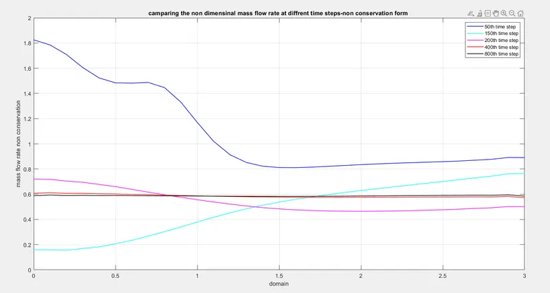
Figure 2:
* The variation of non consarvation mass flow rate againt the diffrent time steps and the variation is same
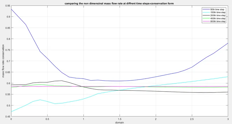
Figure 3:
* The variation of density,time,velocity and mach number at trottle with respect the given time step.
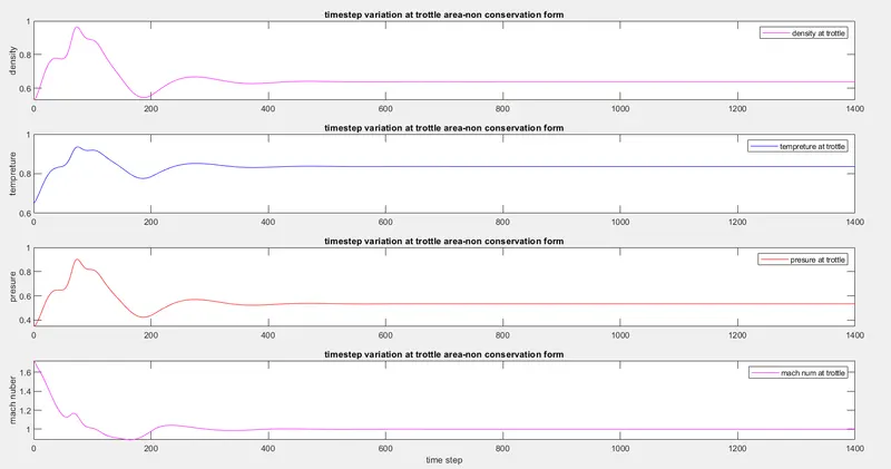
Figure 4:
* the varion of variables with respect to the nozzel lenth of the non conservation form.
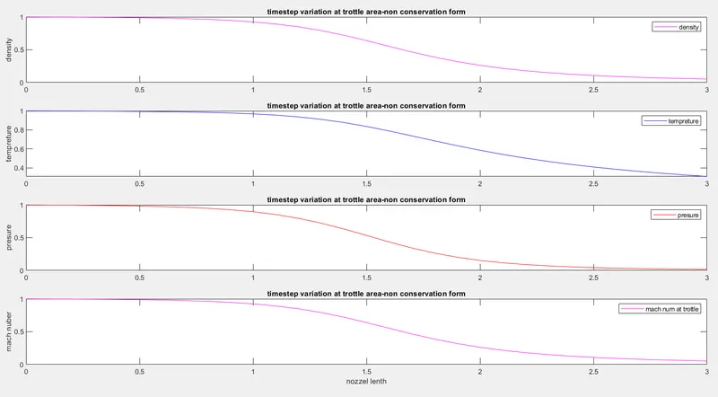
Figure 5:
* The varion of variables with respect to the nozzel lenth of the conservation form.
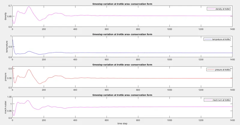
Figure 6:
* The varion of variables with respect to the nozzel lenth of the conservation form.
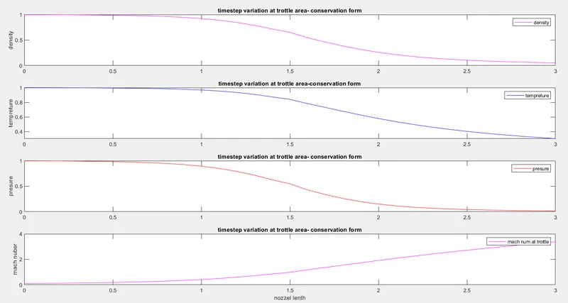
Figure 7:
* The mass flow rate comparition of conservation and non conservation form.