Week 3.5 - Deriving 4th order approximation of a 2nd order derivative using Taylor Table method
FUNCTIONS FOR CENTRAL DIFFERENCE FOURTH ORDER ERROR AT PARTICULAR SPACING 'DX':
% Creating function for the 4th order approximation of the second-order; derivative using central difference; function error_central_differencing = central_difference(x,dx) % Analytical function f(x) = exp(x)*cos(x); % f''(x) = -2*exp(x)*sin(x); analytical_derivative = -2*exp(x)*sin(x); % values of coefficients calculated from our Taylor table; a=-0.083333; b=1.333333; c=-2.500000; d=1.333333; e=-0.083333; % numerical derivative; % central differencing = % ((a*f(x-2*dx))+(b*f(x-dx))+(c*f(x))+(d*f(x+dx))+(e*f(x+2*dx)))/dx^2; %central difference fourth order approximation; central_differencing_fourth_order_approx = ((a*exp(x-2*dx)*cos(x-2*dx))+(b*exp(x-dx)*cos(x-dx))+(c*exp(x)*cos(x))+(d*exp(x+dx)*cos(x+dx))+(e*exp(x+2*dx)*cos(x+2*dx)))/dx^2; error_central_differencing = abs(central_differencing_fourth_order_approx-analytical_derivative); end FUNCTIONS FOR SKEWED RIGHT DIFFERENCE FOURTH ORDER ERROR AT PARTICULAR SPACING 'DX':
% Creating function for the 4th order approximation of the second-order derivative using skewed right-sided difference; function error_skewed_right_sided=skewed_right_sided(x,dx) % analytical function f(x)=exp(x)*cos(x); %f''(x)=-2*exp(x)*sin(x); analytical_derivative=-2*exp(x)*sin(x); %values of coefficients calculated from our Taylor table; a=3.75000; b=-12.83333; c=17.83333; d=-13.00000; e=5.08333; g=-0.83333; %numerical derivative; %skewed right-sided differencing=((a*f(x))+(b*f(x+dx))+(c*f(x+2*dx))+(d*f(x+3*dx))+(e*f(x+4*dx))+(g*f(x+5*dx)))/dx^2; %skewed right-sided fourth order approximation; skewed_right_sided_fourth_order_approx=((a*exp(x)*cos(x))+(b*exp(x+dx)*cos(x+dx))+(c*exp(x+2*dx)*cos(x+2*dx))+(d*exp(x+3*dx)*cos(x+3*dx))+(e*exp(x+4*dx)*cos(x+4*dx))+ (g*exp(x+5*dx)*cos(x+5*dx)))/dx^2; error_skewed_right_sided=abs(skewed_right_sided_fourth_order_approx-analytical_derivative); end FUNCTIONS FOR SKEWED LEFT DIFFERENCE FOURTH ORDER ERROR AT PARTICULAR SPACING 'DX':
% Creating function for the 4th order approximation of the second-order derivative using skewed left-sided difference; function error_skewed_left_sided=skewed_left_sided(x,dx) % analytical function f(x)=exp(x)*cos(x); %f''(x)=-2*exp(x)*sin(x); analytical_derivative=-2*exp(x)*sin(x); %values of coefficients calculated from our Taylor table; a=-0.83333; b=5.08333; c=-13.00000; d=17.83333; e=-12.83333; g=3.75000; %numerical derivative; %skewed left-sided differencing=((a*f(x-5*dx))+(b*f(x-4*dx))+(c*f(x-3*dx))+(d*f(x-2*dx))+(e*f(x-dx))+(g*f(x)))/dx^2; %skewed left-sided fourth order approximation; skewed_left_sided_fourth_order_approx=((a*exp(x-5*dx)*cos(x-5*dx))+(b*exp(x-4*dx)*cos(x-4*dx))+(c*exp(x-3*dx)*cos(x-3*dx))+(d*exp(x-2*dx)*cos(x-2*dx))+(e*exp(x-dx)*cos(x-dx))+ (g*exp(x)*cos(x)))/dx^2; error_skewed_left_sided=abs(skewed_left_sided_fourth_order_approx-analytical_derivative); end MAIN PROGRAM:
%calculating 4th order error of second-order derivative using central, skewed right-sided and left-sided scheme clear allclose allclc x=pi/3;dx=linspace(pi/4,pi/40000,40); %creating 'for' loop; for i=1:length(dx) central_difference_error(i)=central_difference(x,dx(i)); skewed_right_side_error(i)=skewed_right_sided(x,dx(i)); skewed_left_side_error(i)=skewed_left_sided(x,dx(i));end %plotting graphs for dx vs errors for central, skewed right-sided, & skewed left-sided approximations figure(1)plot(dx,central_difference_error,'linewidth',2)hold ongrid onplot(dx,skewed_right_side_error,'r','linewidth',2)hold onplot(dx,skewed_left_side_error,'g','linewidth',2)xlabel('dx')ylabel('error')legend('Central Difference Error','Skewed Right-Sided Error','Skewed Left-Sided Error') figure(2)loglog(dx,central_difference_error,'linewidth',2)hold ongrid onloglog(dx,skewed_right_side_error,'r','linewidth',2)hold onloglog(dx,skewed_left_side_error,'g','linewidth',2)xlabel('dx')ylabel('error')legend('Central Difference Error','Skewed Right-Sided Error','Skewed Left-Sided Error') ERROR FACING:
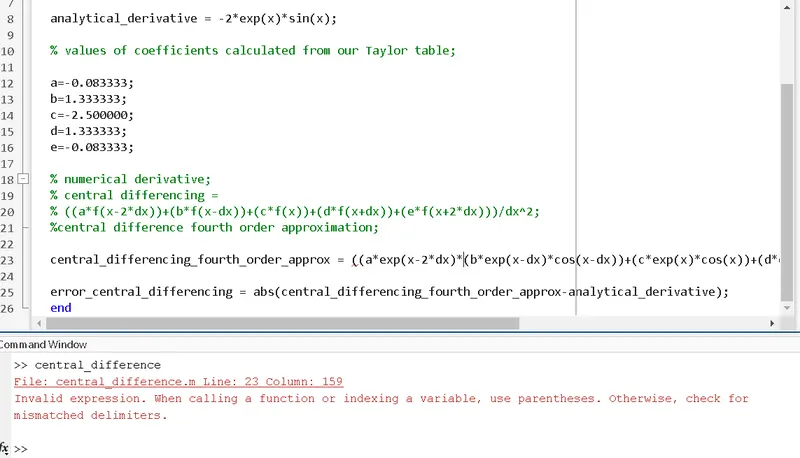
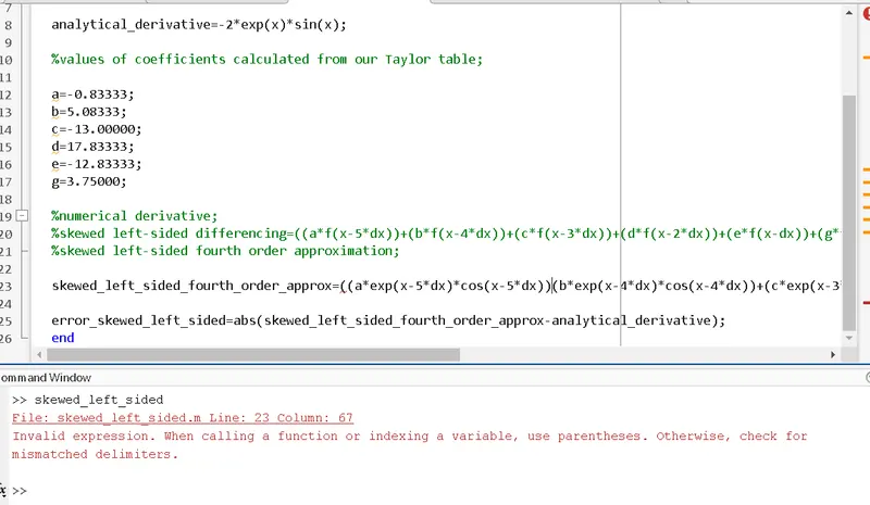
OUTPUTS:
Figure 1:
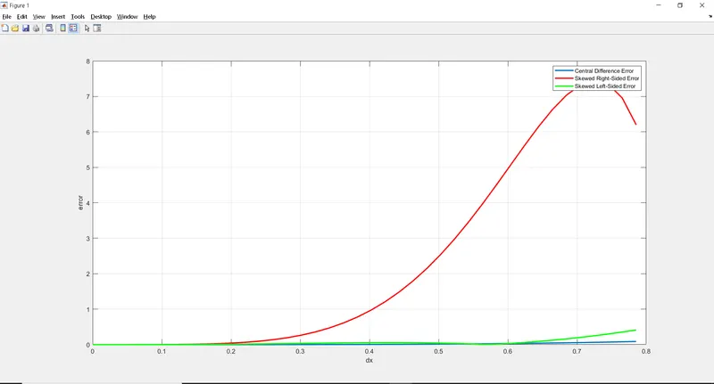
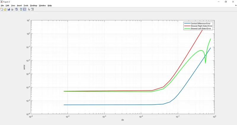
Figure 2:
EXPLANATIONS:
* First of all we create a functions we have save our main program in the same directory in which we have saved our three functions; central difference, skewed right nsided, skewed left sided.
* Then create an array for the range of ‘dx’. We’ll use ‘for loop’ over the range of ‘dx’ and using the functions central, skewed right-sided and skewed left-sided difference fourth order error at a given point (x, dx),
* Now we can move through main program for calculating fourth order error of second-order derivative using central, skewed right-sided and left-sided scheme.let start with clear all close all clc.then arrange the central, skewed right-sided and skewed left-sided difference in for loop.
* then alloted for ploting the axis and label it for both x and y axis and legend and title it for neat presentation.finally run the program i face some of the minor problems .then clear it for a second then ru the output for two figure as named figure 1 and figure 2.After analyzing the graph between ‘error’ vs. ‘dx’ for central, skewed right-sided, and skewed left-sided difference fourth order error.we can easily notice that central difference approximation produces more accurate solutions. hence produces lesser errors as compared to right-skewed and left-skewed difference schemes.
In your own words, describe why a skewed scheme is useful? What can a skewed scheme do that a CD scheme cannot?
* we can see that the central differencing scheme gives us more immaculate solutions or lesser errors as compared to the skewed difference scheme.
* It is not always viable to use the central differencing to evaluate solutions.
* we want to compute numerical approximations for a function at the boundary or corner node; we cannot use the central difference scheme at this particular situation because it requires data from both sides of the node or boundary.
* In this situation skewed difference method plays a major role; as in the skewed scheme data from one side can be used to compute numerical approximation at a point.