Week 7 - Simulation of a 1D Super-sonic nozzle flow simulation using Macormack Method

Aim

 Simulating quasi 1-D supersonic flow through a converging diverging nozzle using MacCormack method

Objective

• Deducing the conservative and non-conservative forms of governing equations and implementing MacCormack method to solve the equations and comparing the results.
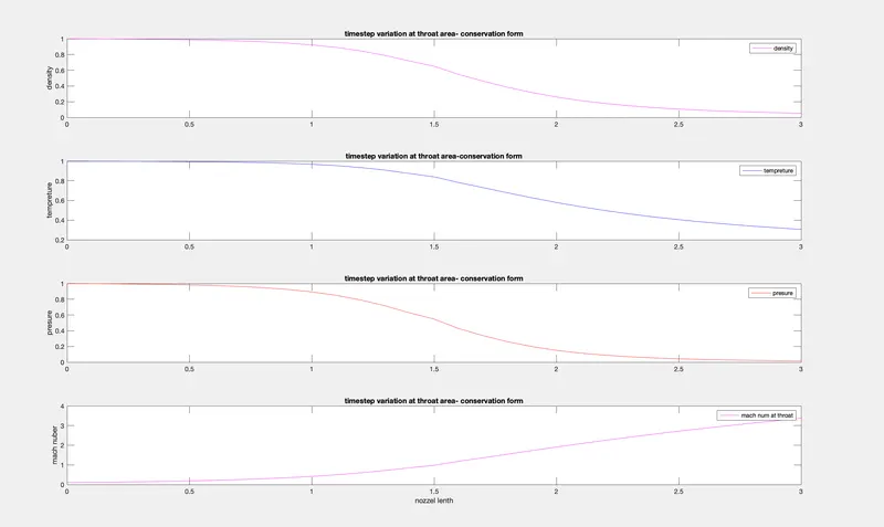
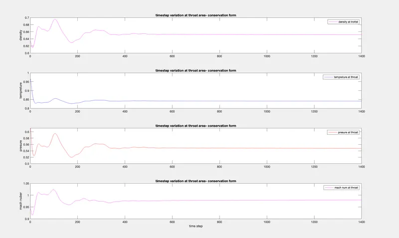
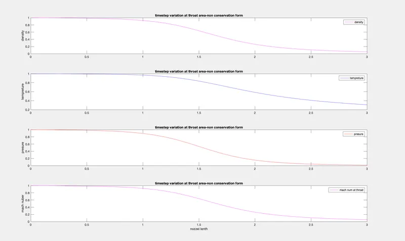
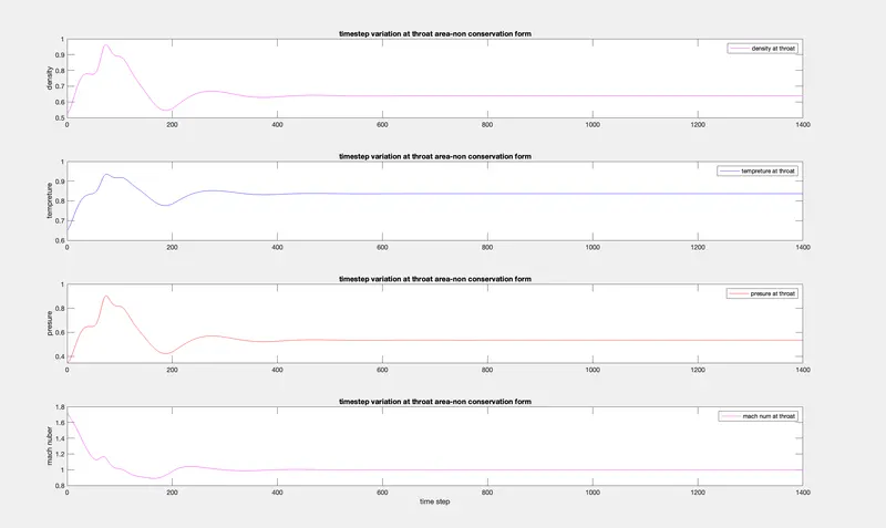
• Computing the steady state distribution of fluid variables in the nozzle and the time variation of the variables.
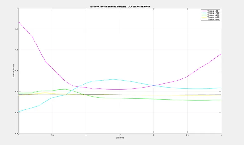
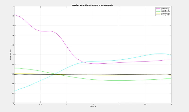
• Studying the variation of mass flow rate inside the nozzle at different time steps under influence of time marching.

Theory

A nozzle is a type of device designed to control the direction or characteristics of fluid flow at the exit of a pipe (or such system). A nozzle is often a pipe or tube of varying cross-sectional area, thus can be used to direct or modify flow of a fluid.

A convergent-divergent nozzle (also known as CD nozzle or de Laval nozzle) is a device used to accelerate a hot, pressurized gas passing through it to a higher supersonic speed in the axial direction by converting heat energy of the flow to kinetic energy. Hence, such nozzles are widely used in steam turbines, supersnic jet engines and rocket engine nozzles. Its operation relies on the different properties of gases flowing at subsonic, sonic and supersonic speeds.

In the field of CFD, MacCormack method is a prominent discretization scheme for obtaining numerical solutions of hyperbolic partial differential equations. (based on second-order finite difference method). It is the variation of two-step Lax-Wendroff scheme but much simple in application.

In this project, the problem is taken from JD Anderson's book on CFD.

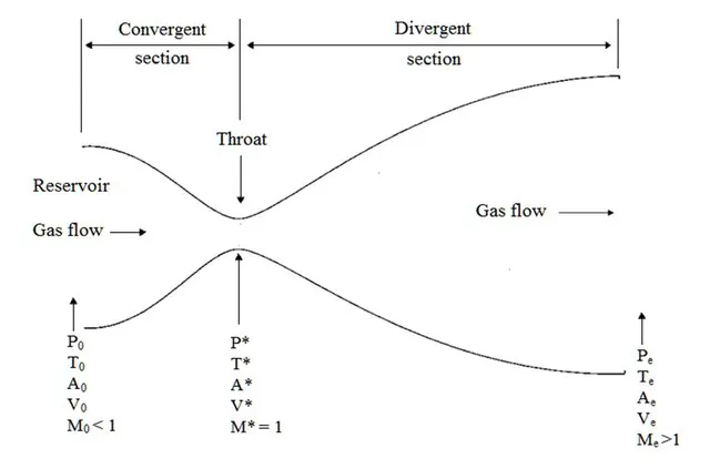
The symmetrical area function for the CD nozzle is given as,

(AA∗)2=1+2.2(x-1.5)2">(AA∗)2=1+2.2(x−1.5)2(AA∗)2=1+2.2(x-1.5)2 @ 0≤x≤3">0≤x≤30≤x≤3

where, A∗">A∗A∗ is the area at the throat of the nozzle and x">xx is the distance along the length of the nozzle.

The non-dimensionalized form of the variables required for this problem are,

x′=xL; V′=Va0; t′=tLa0; ρ′=ρρ0; T′=TT0; p′=pp0; A′=AA∗">x'=xL; V'=Va0; t'=tLa0; ρ'=ρρ0; T'=TT0; p'=pp0; A'=AA∗x′=xL; V′=Va0; t′=tLa0; ρ′=ρρ0; T′=TT0; p′=pp0; A′=AA∗

Governing Equations:

1. Non-Conservative form

The non-conservative form of the governing equation which represent continuity, momentum and energy in terms of non-dimensionless variables,

Continuity: ∂ρ′∂t′=-ρ′∂V′∂x′-ρ′V′∂(lnA′)∂x′-V′∂ρ′∂x′">∂ρ'∂t'=−ρ'∂V'∂x'−ρ'V'∂(lnA')∂x'−V'∂ρ'∂x'∂ρ′∂t′=-ρ′∂V′∂x′-ρ′V′∂(lnA′)∂x′-V′∂ρ′∂x′

Momentum: ∂V′∂t′=-V′∂V′∂x′-1γ[∂T′∂x′+T′ρ′∂ρ′∂x′]">∂V'∂t'=−V'∂V'∂x'−1γ[∂T'∂x'+T'ρ'∂ρ'∂x']∂V′∂t′=-V′∂V′∂x′-1γ[∂T′∂x′+T′ρ′∂ρ′∂x′]

Energy: ∂T′∂t′=-V′∂T′∂x′-(γ-1)T′[∂V′∂x′+V′∂(lnA′)∂x′]">∂T'∂t'=−V'∂T'∂x'−(γ−1)T'[∂V'∂x'+V'∂(lnA')∂x']∂T′∂t′=-V′∂T′∂x′-(γ-1)T′[∂V′∂x′+V′∂(lnA′)∂x′]

The initial conditions as provided in problem statement were,

ρ′(t=0)=1-0.3146x′">ρ'(t=0)=1−0.3146x'ρ′(t=0)=1-0.3146x′
T′(t=0)=1-0.2314x′">T'(t=0)=1−0.2314x'T′(t=0)=1-0.2314x′
V′(t=0)=(0.1+1.09x′)T′(t=0)">V'(t=0)=(0.1+1.09x')√T'(t=0)V′(t=0)=(0.1+1.09x′)T′(t=0)

2. Conservative Form

The conservative form of governing equation which represents continuity, momentum and energy in non-dimensionalized form is given as,

Continuity: ∂(ρ′A′)∂t′+∂(ρ′A′V′)∂x′=0">∂(ρ'A')∂t'+∂(ρ'A'V')∂x'=0∂(ρ′A′)∂t′+∂(ρ′A′V′)∂x′=0

Momentum: ∂(ρ′A′V′)∂t′+∂(ρ′A′V′2+(1γ)p′A′)∂x′=1γp′∂A′∂x′">∂(ρ'A'V')∂t'+∂(ρ'A'V'2+(1γ)p'A')∂x'=1γp'∂A'∂x'∂(ρ′A′V′)∂t′+∂(ρ′A′V′2+(1γ)p′A′)∂x′=1γp′∂A′∂x′

Energy: ∂[ρ′(T′γ-1+γ2V′2)A′]∂t′+∂[ρ′(T′γ-1+γ2V′2)V′A′+p′A′V′]∂x′=0">∂[ρ'(T'γ−1+γ2V'2)A']∂t'+∂[ρ'(T'γ−1+γ2V'2)V'A'+p'A'V']∂x'=0∂[ρ′(T′γ-1+γ2V′2)A′]∂t′+∂[ρ′(T′γ-1+γ2V′2)V′A′+p′A′V′]∂x′=0

In order to simplify these equations, we substitute the following terms, which include the solution vectors Ui">UiUi, the flux vectors Fi">FiFi and the source term J2">J2J2.

U1=ρ′A′">U1=ρ'A'U1=ρ′A′
U2=ρ′A′V′">U2=ρ'A'V'U2=ρ′A′V′
U3=ρ′[T′γ-1+γ2V′2]A′">U3=ρ'[T'γ−1+γ2V'2]A'U3=ρ′[T′γ-1+γ2V′2]A′
F1=ρ′A′V′=U2">F1=ρ'A'V'=U2F1=ρ′A′V′=U2
F2=ρ′A′V′2+1γp′A′=U22U1+γ-1γ[U3-γ2U22U1]">F2=ρ'A'V'2+1γp'A'=U22U1+γ−1γ[U3−γ2U22U1]F2=ρ′A′V′2+1γp′A′=U22U1+γ-1γ[U3-γ2U22U1]
F3=ρ′(T′γ-1+γ2V′2)V′A′+p′A′V′=γU2U3U1-γ(γ-1)2U23U12">F3=ρ'(T'γ−1+γ2V'2)V'A'+p'A'V'=γU2U3U1−γ(γ−1)2U32U21F3=ρ′(T′γ-1+γ2V′2)V′A′+p′A′V′=γU2U3U1-γ(γ-1)2U23U12
J2=1γp′∂A′∂x′">J2=1γp'∂A'∂x'J2=1γp′∂A′∂x′

After substituting these terms in governing equations, we have,

∂U1∂t′=-∂F1∂x′">∂U1∂t'=−∂F1∂x'∂U1∂t′=-∂F1∂x′
∂U2∂t′=-∂F2∂x′+J2">∂U2∂t'=−∂F2∂x'+J2∂U2∂t′=-∂F2∂x′+J2
∂U3∂t′=-∂F3∂x′">∂U3∂t'=−∂F3∂x'∂U3∂t′=-∂F3∂x′

The flow variables are calculated on numerical solution of the above terms as,

ρ′=U1A′">ρ'=U1A'ρ′=U1A′
V′=U2U1">V'=U2U1V′=U2U1
T′=(γ-1)[U3U1-γ2V′2]">T'=(γ−1)[U3U1−γ2V'2]T′=(γ-1)[U3U1-γ2V′2]
p′=ρ′T′">p'=ρ'T'p′=ρ′T′

The initial conditions as provided in the problem statement are,

ρ′(t=0)={1.0for0≤x′<0.5(1.0-0.366(x′-0.5))for0.5≤x′<1.5(0.634-0.3879(x′-1.5))for1.5≤x′≤3">ρ'(t=0)=⎧⎪⎨⎪⎩1.0for0≤x'<0.5(1.0−0.366(x'−0.5))for0.5≤x'<1.5(0.634−0.3879(x'−1.5))for1.5≤x'≤3ρ′(t=0)={1.0for0≤x′<0.5(1.0-0.366(x′-0.5))for0.5≤x′<1.5(0.634-0.3879(x′-1.5))for1.5≤x′≤3

T′(t=0)={1.0for0≤x′<0.5(1.0-0.167(x′-0.5))for0.5≤x′<1.5(0.833-0.3507(x′-1.5))for1.5≤x′≤3">T'(t=0)=⎧⎪⎨⎪⎩1.0for0≤x'<0.5(1.0−0.167(x'−0.5))for0.5≤x'<1.5(0.833−0.3507(x'−1.5))for1.5≤x'≤3T′(t=0)={1.0for0≤x′<0.5(1.0-0.167(x′-0.5))for0.5≤x′<1.5(0.833-0.3507(x′-1.5))for1.5≤x′≤3

V′(t=0)=U2ρ′(t=0)A′=0.59ρ′(t=0)A′">V'(t=0)=U2ρ'(t=0)A'=0.59ρ'(t=0)A'V′(t=0)=U2ρ′(t=0)A′=0.59ρ′(t=0)A′ (considering a constant mass flow rate of U2=ρ′A′V′=0.59">U2=ρ'A'V'=0.59U2=ρ′A′V′=0.59 just for the initial condition)

MacCormack method of solving:

The MacCormack numerical scheme is a common method to solve flow equations. It basically consists of four steps:

1. Predictor step
2. Intermediate solution update
3. Corrector step
4. Final solution update

In the predictor step, the spatial derivative are calculated using the forward difference scheme. This time derivative from the governing equations obtained is recorded as ∂u(∂t)p">∂u(∂t)p∂u(∂t)p. Consider, the continuity equation for the non-conservative form. From the predictor step, we obtain,

(∂ρi∂t)P=-ρ′i[V′i+1-V′iΔx′]-ρ′iV′i[(ln(A′i+1-ln(A′i))Δx′]-V′i[ρ′i+1-ρ′iΔx′]">(∂ρi∂t)P=−ρ'i[V'i+1−V'iΔx']−ρ'iV'i[(ln(A'i+1−ln(A'i))Δx']−V'i[ρ'i+1−ρ'iΔx'](∂ρi∂t)P=-ρ′i[V′i+1-V′iΔx′]-ρ′iV′i[(ln(A′i+1-ln(A′i))Δx′]-V′i[ρ′i+1-ρ′iΔx′]

During the intermediate solution update, the variable is updated based on the time derivative obtained from the predictor step as:

ρi,Pt+Δt=ρ′i+(∂ρ′i∂t′)PΔt">ρt+Δti,P=ρ'i+(∂ρ'i∂t')PΔtρi,Pt+Δt=ρ′i+(∂ρ′i∂t′)PΔt

Using these updated values, the governing equations are solved again using backward differencing in space in the corrector step. The time-derivative obtained during the corrector step is stored as (∂u∂t)C">(∂u∂t)C(∂u∂t)C.

(∂ρi∂t)C=-ρ′i,P[V′i,P-V′i-1,PΔx′]-ρ′i,PV′i,P[(ln(A′i,P-ln(A′i-1,P))Δx′]-V′i,P[ρ′i,P-ρ′i-1,PΔx′]">(∂ρi∂t)C=−ρ'i,P[V'i,P−V'i−1,PΔx']−ρ'i,PV'i,P[(ln(A'i,P−ln(A'i−1,P))Δx']−V'i,P[ρ'i,P−ρ'i−1,PΔx'](∂ρi∂t)C=-ρ′i,P[V′i,P-V′i-1,PΔx′]-ρ′i,PV′i,P[(ln(A′i,P-ln(A′i-1,P))Δx′]-V′i,P[ρ′i,P-ρ′i-1,PΔx′]

For the final solution update, we use the average of the time-derivatives obtained using the predictor and the corrector steps. Since we are using forward difference in predictor step and backward difference in corrector step, the average of the time-derivative for the final update, the overall scheme becomes a second order numerical scheme.

(∂ρ∂t)av=12[(∂ρ∂t)P+(∂ρ∂t)C]">(∂ρ∂t)av=12[(∂ρ∂t)P+(∂ρ∂t)C](∂ρ∂t)av=12[(∂ρ∂t)P+(∂ρ∂t)C]

ρit+Δt=ρit+(∂ρ∂t)avΔt">ρt+Δti=ρti+(∂ρ∂t)avΔt

MAIN CODE

% writing program for simulation of 1D NOZZLE SUPERSONIC FLOW USING MACCORMAC'S METHOD 

clear all
close all
clc

%defing the inputs 
% number of grids points

n=31;
x=linspace(0,3,n);
dx=x(2)-x(1);


gamma=1.4;

% numbers of time steps

nt=1400;
CFL=0.5;

% defing the function for non conservation form of simulation 

tic;
[mass_flow_rate_nc, presure_nc, mach_num_nc, rho_nc, v_nc, T_nc, rho_throat_nc, v_throat_nc, T_throat_nc, mass_flow_rate_throat_nc, presure_throat_nc, mach_num_throat_nc]=non_conservative(x,dx,n,gamma,nt,CFL)
time_elapsed=toc;
fprintf('time elapesed for non coservation form:%f',time_elapsed)
hold on 

%ploting the graphs

figure(3)

%for density

subplot(4,1,1)
plot(linspace(1,nt,1400),rho_throat_nc,"Color","m");
ylabel("density")
legend({'density at throat'})
title('timestep variation at throat area-non conservation form')

%for tempreture 

subplot(4,1,2)
plot(linspace(1,nt,1400),T_throat_nc,"Color","b");
ylabel("tempreture")
legend({'tempreture at throat'})
title('timestep variation at throat area-non conservation form')

% for pressure

subplot(4,1,3)
plot(linspace(1,nt,1400),presure_throat_nc,"Color","r");
ylabel("presure")
legend({'presure at throat'})
title('timestep variation at throat area-non conservation form')

% for mach number 

subplot(4,1,4)
plot(linspace(1,nt,1400),mach_num_throat_nc,"Color","m");
xlabel('time step')
ylabel("mach nuber")
legend({'mach num at throat'})
title('timestep variation at throat area-non conservation form')


% steadystate simulation for primitive value for nom conservation form 

figure(4)

%for density

subplot(4,1,1)
plot(x,rho_nc,"Color","m");
ylabel("density")
legend({'density'})
title('timestep variation at throat area-non conservation form')

% for tempreture 

subplot(4,1,2)
plot(x,T_nc,"Color","b");
ylabel("tempreture")
legend({'tempreture'})
title('timestep variation at throat area-non conservation form')

% for presure

subplot(4,1,3)
plot(x,presure_nc,"Color","r");
ylabel("presure")
legend({'presure'})
title('timestep variation at throat area-non conservation form')

% for mach number
 
subplot(4,1,4)
plot(x,rho_nc,"Color","m");
xlabel('nozzel lenth')
ylabel("mach nuber")
legend({'mach num at throat'})
title('timestep variation at throat area-non conservation form')

% defing the function for conservation form of simulation
 
tic;
[mass_flow_rate_c, presure_c, mach_num_c, rho_c,v_c, T_c, rho_throat_c, v_throat_c, T_throat_c, mass_flow_rate_throat_c, presure_throat_c, mach_num_throat_c]=Conservative(x,dx,n,gamma,nt,CFL);
time_elapsed_c=toc;
fprintf('time elapesed for coservation form:%f',time_elapsed_c)
hold on 

% plotting
 
figure(5)

% for density

subplot(4,1,1)
plot(linspace(1,nt,1400),rho_throat_c,'Color','m');
ylabel("density")
legend({'density at trottel'})
title('timestep variation at throat area- conservation form')

% for tempreture 

subplot(4,1,2)
plot(linspace(1,nt,1400),T_throat_c,'Color',"b");
ylabel("tempreture")
legend({'tempreture at throat'})
title('timestep variation at throat area- conservation form')

% for presure

subplot(4,1,3)
plot(linspace(1,nt,1400),presure_throat_c,"Color","r");
ylabel("presure")
legend({'presure at throat'})
title('timestep variation at throat area- conservation form')

% for mach number
 
subplot(4,1,4)
plot(linspace(1,nt,1400),mach_num_throat_c,"Color","m");
xlabel('time step')
ylabel("mach nuber")
legend({'mach num at throat'})
title('timestep variation at throat area- conservation form')


% steady sTATE simulation for primitive value for nom conservation form
 
figure(6)

% for density

subplot(4,1,1)
plot(x,rho_c,"Color","m");
ylabel("density")
legend({'density'})
title('timestep variation at throat area- conservation form')



% for temperature
 
subplot(4,1,2)
plot(x,T_c,"Color","b");
ylabel("tempreture")
legend({'tempreture'})
title('timestep variation at throat area-conservation form')

% for pressure

subplot(4,1,3)
plot(x,presure_c,"Color","r");
ylabel("presure")
legend({'presure'})
title('timestep variation at throat area- conservation form')

%for mach number
 
subplot(4,1,4)
plot(x,mach_num_c,"Color","m");
xlabel('nozzel lenth')
ylabel("mach nuber")
legend({'mach num at throat'})
title('timestep variation at throat area- conservation form')


%camparing the plots of narmalization mass flow rate of both forms

figure(7)
hold on 
plot(x,mass_flow_rate_nc,'r','linewidth',2)
hold on 
plot(x,mass_flow_rate_c,'b','linewidth',2)
hold on 
grid on
legend('non conversion','conversion')
xlabel('lenght of the domain')
ylabel('mass flow rate')
title('camparison of narmalization mass flow rate of both forms')
 

FUNCTION CODE FOR CONSERVATIVE

function [mass_flow_rate_c, presure_c, mach_num_c, rho_c, v_c, T_c, rho_throat_c, v_throat_c, T_throat_c, mass_flow_rate_throat_c, presure_throat_c, mach_num_throat_c]=conservative(x,dx,n,gamma,nt,CFL)

%[mass_flow_rate_c, pressure_c, mach_num_c, rho_c, v_c, T_c, rho_throat_c, v_throat_c, T_throat_c, mass_flow_rate_throat_c, presure_throat_c, mach_num_throat_c]=conservation_form(x,dx,n,gamma,nt,CFL);

%defining the intial  condition for density and tempreture

for m =1:n
    if(x(m) >=0 && x(m) <=0.5)
        rho_c(m)=1;
        T_c(m) =1;
    elseif (x(m) >=0.5 && x(m) <=1.5)
        rho_c(m)=1-0.366*(x(m)-0.5);
        T_c(m) =1-0.167*(x(m)-0.5);
    elseif  (x(m) >=1.5 && x(m) <=3.5)
         rho_c(m)=0.634-0.3879*(x(m)-1.5);
        T_c(m) =0.833-0.3507*(x(m)-1.5);
    end
end

%defining for velocity

a=1+2.2*(x-1.5).^2;
v_c =0.59./(rho_c.*a);
presure_c=rho_c.*T_c;

% defining the throat 

throat = find(a==1);

% defing the initiel solution variabels
 
U1 =rho_c.*a;
U2 =rho_c.*a.*v_c;
U3 =rho_c.*a.*(T_c./(gamma-1))+((gamma/2).*v_c.^2);

%defining the time loop


for k =1:nt

    %defining the time step

    dt =min(CFL.*dx./(sqrt(T_c)+v_c));

    %defing the old values 

    U1_old=U1;
    U2_old=U2;
    U3_old=U3;

    %calculating the flux

    F1=U2;
    F2=((U2.^2)./U1)+((gamma-1)/gamma)*(U3-(gamma/2)*((U2.^2)./U1));
    F3=((gamma*U2.*U3)./U1)-(gamma*(gamma-1)*((U2.^3)./(2*U1.^2)));

    % calculatinf the predector method 

    for j = 2:n-1

        % calculating the souse term

        J2(j)=(1/gamma)*rho_c(j)*T_c(j)*((a(j+1)-a(j))/dx);

        % continuity eqution 

        dU1_dt_p(j)=-((F1(j+1)-F1(j))/dx);

        % momentum equation 

         dU2_dt_p(j)=-((F2(j+1)-F2(j))/dx)+J2(j);
        

         %energy equation
 
          dU3_dt_p(j)=-((F3(j+1)-F3(j))/dx);

          % updating the soluton vector
 
          U1(j)=U1(j)+dU1_dt_p(j)*dt;
          U2(j)=U2(j)+dU2_dt_p(j)*dt;
          U3(j)=U3(j)+dU3_dt_p(j)*dt;
    end

    %updating the flux 

    F1=U2;
    F2=((U2.^2)./U1)+((gamma-1)/gamma)*(U3-(gamma*0.5*(U2.^2)./U1));
    F3=((gamma*U2.*U3)./U1)-((gamma*0.5*(gamma-1)*(U2.^3)./(U1.^2)));

   

    % know calculating for corrector method

    for j=2:n-1

% calculating the souse term

        J2(j)=(1/gamma)*rho_c(j)*T_c(j)*((a(j)-a(j-1))/dx);

        % continuty eqution 

        dU1_dt_c(j)=-((F1(j)-F1(j-1))/dx);

        % momentum equation
 
         dU2_dt_c(j)=-((F2(j)-F2(j-1))/dx)+J2(j);
        

         %energy equation 

          dU3_dt_c(j)=-((F3(j)-F3(j-1))/dx);

    end

    %computing the avarege value 

    dU1_dt_av=0.5*(dU1_dt_p+dU1_dt_c);
    dU2_dt_av=0.5*(dU2_dt_p+dU2_dt_c);
    dU3_dt_av=0.5*(dU3_dt_p+dU3_dt_c);

    % calculating the final solution 

    for m=2:n-1
        U1(m)=U1_old(m)+dU1_dt_av(m)*dt;
        U2(m)=U2_old(m)+dU2_dt_av(m)*dt;
        U3(m)=U3_old(m)+dU3_dt_av(m)*dt;
    end

    %appliying the boundry conditions at inlets 

    U1(1)=rho_c(1)*a(1);
    U2(1)=2*U2(2)-U2(3);
    v_c(1)=U2(1)./U1(1);
    U3(1)=U1(1)*((T_c(1)/(gamma-1))+((gamma/2)*(v_c(1)).^2));

    %at outlet

     U1(n)=2*U1(n-1)-U1(n-2);
     U2(n)=2*U2(n-1)-U2(n-2);
     U3(n)=2*U3(n-1)-U3(n-2);

     %final primitive value update

     rho_c=U1./a;
     v_c=U2./U1;
     T_c=(gamma-1)*((U3./U1)-(gamma/2)*(v_c).^2);

     % defing the mass flow rate 

        %defing the flow rate 

        mass_flow_rate_c = rho_c.*a.*v_c;
        presure_c = rho_c.*T_c;
        mach_num_c = (v_c./sqrt(T_c));

        % calculating the variables at throat
 
        rho_throat_c(k) = rho_c(throat);
        T_throat_c(k) = T_c(throat);
        v_throat_c(k) = v_c(throat);
        mass_flow_rate_throat_c(k) =  mass_flow_rate_c(throat);
        presure_throat_c(k) = presure_c(throat);
        mach_num_throat_c(k) = mach_num_c(throat);

    %PLOTTING
    %Comparison of non-dimensional Mass flow rates at different time steps
    figure(2)
    if k == 50
        plot(x, mass_flow_rate_c, 'm', 'linewidth', 1.25,'DisplayName',['Timestep = ',num2str(k)]);
        hold on
    elseif k == 100
        plot(x, mass_flow_rate_c, 'c', 'linewidth', 1.25,'DisplayName',['Timestep = ',num2str(k)]);
        hold on
    elseif k == 200
        plot(x, mass_flow_rate_c, 'g', 'linewidth', 1.25,'DisplayName',['Timestep = ',num2str(k)]);
        hold on
    elseif k == 400
        plot(x, mass_flow_rate_c, 'y', 'linewidth', 1.25,'DisplayName',['Timestep = ',num2str(k)]);
        hold on
    elseif k == 800
        plot(x, mass_flow_rate_c, 'k', 'linewidth', 1.25,'DisplayName',['Timestep = ',num2str(k)]);
        hold on
    end




end
legend
title('Mass flow rates at different Timesteps - CONSERVATIVE FORM')
xlabel('Distance')
ylabel('Mass flow rate')
axis([0 3 0.4 1])
grid on
end

FUNCTION CODE FOR NON CONSERVATIVE

%writting the function for non conservation form using maccormack method

function [mass_flow_rate_nc, presure_nc, mach_num_nc, rho_nc, v_nc, T_nc, rho_throat_nc, v_throat_nc, T_throat_nc, mass_flow_rate_throat_nc, presure_throat_nc, mach_num_throat_nc]=non_conservative(x,dx,n,gamma,nt,CFL)


%defining the initial boundry condition

rho_nc=1 - 0.3146*x;
T_nc =1 - 0.2341*x;
v_nc=(0.1+1.09*x).*T_nc.^0.5;

%area of the nozzel

a = 1+2.2*(x-1.5).^2;

% defining throat
throat = find(a==1);

%defining the time loop
%defining the nodes

for k =1:nt
    dt =min(CFL.*dx./(sqrt(T_nc)+v_nc));

    %defining the old values

    rho_old=rho_nc;
    T_old=T_nc;
    v_old =v_nc;

    %know we have to solve  for predictor method

    for j =2:n-1
        dv_dx =(v_nc(j+1)-v_nc(j))./dx;
        drho_dx =(rho_nc(j+1)-rho_nc(j))./dx;
        dT_dx =(T_nc(j+1)-T_nc(j))./dx;
        dlog_a_dx =(log(a(j+1))-log(a(j)))./dx;

        % continuty equation
        drho_dt_p(j)=-rho_nc(j)*dv_dx-rho_nc(j)*v_nc(j)*dlog_a_dx-v_nc(j)*drho_dx;

        %momemtum equation

        dv_dt_p(j)=-v_nc(j)*dv_dx-(1/gamma)*(dT_dx+(T_nc(j)*drho_dx/rho_nc(j)));

        % energy equation
        dT_dt_p(j)=-v_nc(j)*dT_dx-(gamma-1)*T_nc(j)*(dv_dx+v_nc(j)*dlog_a_dx);

        % updating the solution
        rho_nc(j)=rho_nc(j)+drho_dt_p(j)*dt;
        v_nc(j)=v_nc(j)+dv_dt_p(j)*dt;
        T_nc(j)=T_nc(j)+dT_dt_p(j)*dt;
    end

    %know we have to define the equations fo corrector methods
    % simplifying  terms there fore we have equation for continity momentum energy in that equation we are descritizing using backword scheme

    for j=2:n-1
        dv_dx =(v_nc(j)-v_nc(j-1))./dx;
        drho_dx =(rho_nc(j)-rho_nc(j-1))./dx;
        dT_dx =(T_nc(j)-T_nc(j-1))./dx;
        dlog_a_dx =(log(a(j))-log(a(j-1)))./dx;

        % continuty equation

        drho_dt_c(j)=-rho_nc(j)*dv_dx-rho_nc(j)*v_nc(j)*dlog_a_dx-v_nc(j)*drho_dx;

        % momemtum equation

        dv_dt_c(j)=-v_nc(j)*dv_dx-(1/gamma)*(dT_dx+(T_nc(j)*drho_dx/rho_nc(j)));

        % energy equation

        dT_dt_c(j)=-v_nc(j)*dT_dx-(gamma-1)*T_nc(j)*(dv_dx+v_nc(j)*dlog_a_dx);
    end




    % computing the averege vtime deravetion or averege solution

    drho_dt_av =0.5.*(drho_dt_p+drho_dt_c);
    dv_dt_av =0.5.*(dv_dt_p+dv_dt_c);
    dT_dt_av =0.5.*(dT_dt_p+dT_dt_c);

    % final solution

    for m=2:n-1
        rho_nc(m)=rho_old(m)+(drho_dt_av(m))*dt;
        v_nc(m)=v_old(m)+(dv_dt_av(m))*dt;
        T_nc(m)=T_old(m)+(dT_dt_av(m))*dt;
    end

    % applying the boundary conditions
    % At inlet

    rho_nc(1)=1;
    v_nc(1)=2*v_nc(2)-v_nc(3);
    T_nc(1)=1;

    % At oulet
    rho_nc(n)=2*rho_nc(n-1)-rho_nc(n-2);
    v_nc(n)=2*v_nc(n-1)-v_nc(n-2);
    T_nc(n)=2*T_nc(n-1)-T_nc(n-2);

    %defining the flow rate

    mass_flow_rate_nc=rho_nc.*a.*v_nc;
    presure_nc=rho_nc.*T_nc;
    mach_num_nc=(v_nc./sqrt(T_nc));

    % calculating the variables at throat
    %throat=find(a==1);

    rho_throat_nc(k) = rho_nc(throat);
    T_throat_nc(k) = T_nc(throat);
    v_throat_nc(k) = v_nc(throat);
    mass_flow_rate_throat_nc(k) = mass_flow_rate_nc(throat);
    presure_throat_nc(k) = presure_nc(throat);
    mach_num_throat_nc(k) = mach_num_nc(throat);


    %plotting
    %comparsion of non-dimensional b/w mass flow rate at differant time step

    figure(1)

    if k == 50
        plot(x, mass_flow_rate_nc, 'm', 'linewidth', 1.25,'DisplayName',['Timestep = ',num2str(k)]);
        hold on
    elseif k == 100
        plot(x, mass_flow_rate_nc, 'c', 'linewidth', 1.25,'DisplayName',['Timestep = ',num2str(k)]);
        hold on
    elseif k == 200
        plot(x, mass_flow_rate_nc, 'g', 'linewidth', 1.25,'DisplayName',['Timestep = ',num2str(k)]);
        hold on
    elseif k == 400
        plot(x, mass_flow_rate_nc, 'y', 'linewidth', 1.25,'DisplayName',['Timestep = ',num2str(k)]);
        hold on
    elseif k == 800
        plot(x, mass_flow_rate_nc, 'k', 'linewidth', 1.25,'DisplayName',['Timestep = ',num2str(k)]);
        hold on
    end
end
legend
title('mass flow rate at differant time step of non conservation ')
xlabel('distance');
ylabel('mass flow rate');
axis([0 3 0 2])
grid on
end

OUTPUT

OBSERVATION AND CONCLUSION

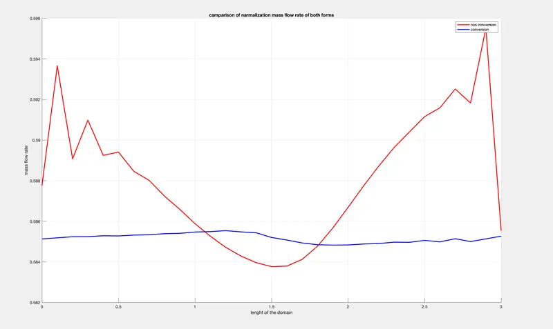
• For comparing the conservative and non-conservative form, the values of the flow variables at the throat of the nozzle are plotted at each time step. It can be observed that at smller time-steps, the behaviour of non-conservative form shows unstable results. (it shows oscillations) but with increase in time step, the difference in conservative and non-conservative approach diminshes.
• If we notice the residuals (average time derivatives of variables) of both the approaches the conservative form converges to a steady state faster than non-conservative form.
• On varying the grid size, it is noted that the conservative form almost maintains its consistency but the non conservative form tends to become stable (on increasing grid size).
• Thus MaCormack method provides quite stable and close to exact solutions, hence, it is widely implemented to solve various flow problems.

REFERENCES