Week 7 - Simulation of a 1D Super-sonic nozzle flow simulation using Macormack Method

Aim:

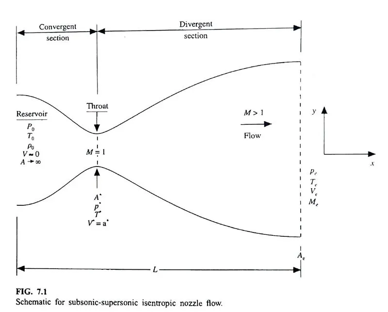
• Simulate the isentropic flow through a quasi 1D subsonic-supersonic nozzle.
• Derive both the conservation and non-conservation forms of the governing equations and solve them using the MacCormack's technique.
• Determine the steady-state temperature distribution for the flow-field variables and investigate the difference between the two forms of governing equations by comparing their solutions.

Show the following plots

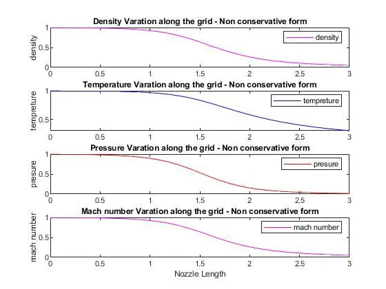
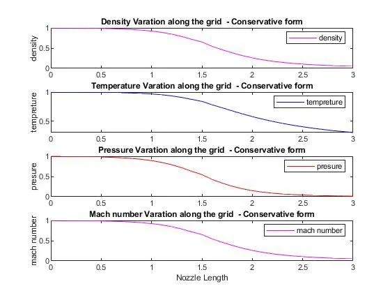
1. Steady-state distribution of primitive variables inside the nozzle
2. Time-wise variation of the primitive variables
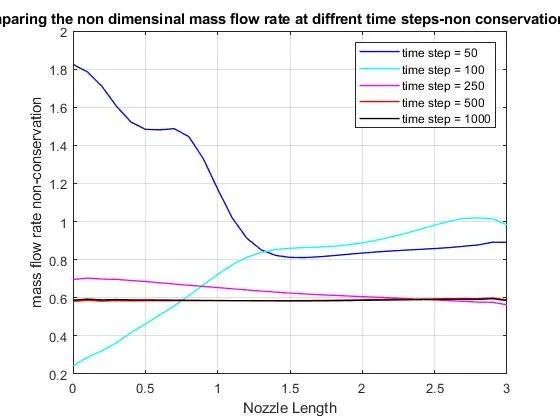
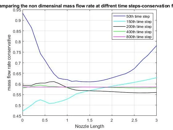
3. Variation of Mass flow rate distribution inside the nozzle at different time steps during the time-marching process
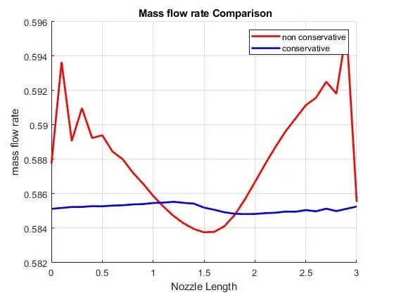
4. Comparison of Normalized mass flow rate distributions of both forms

Theory:

Direct numerical stimulation of fluid flow through nozzle has always been a challenging problem and an area of immense interest for modern engineers. Converging-Diverging nozzle has been extensively used in a wide range of Industrial applications ranging from steam turbines to rocket engine nozzles. The condition for operation so that the nozzle produces supersonic flow is that the Mach number at throat should be equal to one. This condition is known as choked flow. As the fluid expands further in the diverging section, the fluid flow increases to supersonic velocities.(Mach Number>1).If the choke condition is not met, the nozzle simply acts as a Venturi tube and would produce subsonic flow even at the outlet. This paper uses an explicit finite difference scheme for numerical solution of fluid flow. This scheme is fully explicit and second order accurate in both time and space.

There for we have equation to solve this flow shown below:

For non-conservative form:

Continuity equation:

Momentum equation

Energy equation

For Conservative Form:

Continuity Equation:

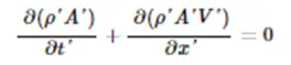
Momentum Equation:

Energy Equation:

McCORMACK'S TECHNIQUE

Let f(x) be the function to be solved. This technique involves 5 steps to be followed in order.

• Initial profile

All the flow field variables are to be determined in this step.

• Predictor step

A predicted derivative is found using the forward differencing scheme.

〖∂f/∂t〗_p=(f(i+1)-i(i))/∆x

Solution update is fp=f_Initial+(∂f/∂t)p⋅Δt

• Corrected Step

A corrected derivative is found using backward differencing scheme

〖 ( ∂f/dt)〗_c=f(i)-f(i-1)/Δx

• Average

Average of the predictor and corrector are found

〖 ( ∂f/dt)〗_avg=0.5(〖 ( ∂f/dt)〗_p+〖 ( ∂f/dt)〗_c)

• Final Solution

fsol=fInitial+(∂f/∂t)avg⋅Δt

Main Code:

clear all
close all
clc
%number of grids points
n=31;
x=linspace(0,3,n);
dx=x(2)-x(1);
gama=1.4;

%numbers of time steps
nt=1400;
CFL=0.5;

%defing the function for non conservation form of simulation 
[mass_flow_rate_nc, presure_nc, mach_num_nc, rho_nc, v_nc, t_nc, rho_t_nc, v_t_nc, t_t_nc, mass_flow_rate_t_nc, presure_t_nc, mach_num_t_nc]=non_conservative_form_original(x,dx,n,gama,nt,CFL)

time_elapsed=toc;
fprintf('time elapesed for non conservative form is %f',time_elapsed)
hold on 
%ploting the graphs
figure(3)
%density
subplot(4,1,1)
plot(linspace(1,nt,1400),rho_t_nc,'Color','m');
xlabel('Time step')
ylabel('Density')
legend({'Density at Throat Section'})
title('Density at Throat Section for Different Time step - Non conservative form')

%tempreture 
subplot(4,1,2)
plot(linspace(1,nt,1400),t_t_nc,'Color','b');
xlabel('Time step')
ylabel('Tempreture')
legend({'Tempreture at Throat Section'})
title('Temperature at Throat Section for Different Time step - Non conservative form')

%pressure
subplot(4,1,3)
plot(linspace(1,nt,1400),presure_t_nc,'Color','r');
xlabel('Time step')
ylabel('Presure')
legend({'Pressure at Throat Section'})
title('Pressure at Throat Section for Different Time step - Non conservative form')

%mach number 
subplot(4,1,4)
plot(linspace(1,nt,1400),mach_num_t_nc,'Color','m');
xlabel('Time step')
ylabel('Mach number')
legend({'Mach number at Throat Section'})
title('Mach Numberat Throat Section for Different Time step - Non conservative form')


% Steady State simulation of primitive value for non- conservative form 
figure(4)
title('Steady State simulation of primitive value for non conservative form ');
%density
subplot(4,1,1)
plot(x,rho_nc,'Color','m');
ylabel('density')
legend({'density'})
title('Density Varation along the grid - Non conservative form')

%tempreture 
subplot(4,1,2)
plot(x,t_nc,'Color','b');
ylabel('tempreture')
legend({'tempreture'})
title('Temperature Varation along the grid - Non conservative form')

% presure
subplot(4,1,3)
plot(x,presure_nc,'Color','r');
ylabel('presure')
legend({'presure'})
title('Pressure Varation along the grid - Non conservative form')

%mach number 
subplot(4,1,4)
plot(x,rho_nc,'Color','m');
xlabel('Nozzle Length')
ylabel('mach number')
legend({'mach number'})
title('Mach number Varation along the grid - Non conservative form')

% %defing the function for conservation form of simulation 
tic;
[mass_flow_rate_c, presure_c, mach_num_c, rho_c, v_c, t_c, rho_t_c, v_t_c, t_t_c, mass_flow_rate_t_c, presure_t_c, mach_num_t_c]=conservation_form(x,dx,n,gama,nt,CFL)
time_elapsed_c=toc;
fprintf('time elapesed for coservative form is %f',time_elapsed_c)
hold on 

%plotting the graphs for conservative form
figure(5)
%density
subplot(4,1,1)
plot(linspace(1,nt,1400),rho_t_c,'Color','m');

ylabel('Density')
legend({'Density at Throat Section'})
title('Density at Throat Section for Different Time step - Conservative form')

%tempreture 
subplot(4,1,2)
plot(linspace(1,nt,1400),t_t_c,'Color','b');

ylabel('Tempreture')
legend({'Tempreture at Throat Section'})
title('Temperature at Throat Section for Different Time step  - Conservative form')

%pressure
subplot(4,1,3)
plot(linspace(1,nt,1400),presure_t_c,'Color','r');

ylabel('Presure')
legend({'Pressure at Throat Section'})
title('Pressure at Throat Section for Different Time step  - Conservative form')

%mach number 
subplot(4,1,4)
plot(linspace(1,nt,1400),mach_num_t_c,'Color','m');
xlabel('Time step')
ylabel('Mach number')
legend({'Mach number at Throat Section'})
title('Mach Numberat Throat Section for Different Time step  - Conservative form')


% Steady State simulation of primitive value for conservative form 
figure(6)
%density
subplot(4,1,1)
plot(x,rho_c,'Color','m');
ylabel('density')
legend({'density'})
title('Density Varation along the grid  - Conservative form')

%tempreture 
subplot(4,1,2)
plot(x,t_c,'Color','b');
ylabel('tempreture')
legend({'tempreture'})
title('Temperature Varation along the grid  - Conservative form')

% presure
subplot(4,1,3)
plot(x,presure_c,'Color','r');
ylabel('presure')
legend({'presure'})
title('Pressure Varation along the grid  - Conservative form')

%mach number 
subplot(4,1,4)
plot(x,rho_c,'Color','m');
xlabel('Nozzle Length')
ylabel('mach number')
legend({'mach number'})
title('Mach number Varation along the grid  - Conservative form')



%camparing the plots of narmalization mass flow rate of both forms

figure(7)
hold on 
plot(x,mass_flow_rate_nc,'r','linewidth',2)
hold on 
plot(x,mass_flow_rate_c,'b','linewidth',2)
hold on 
grid on
legend('non conservative','conservative')
xlabel('Nozzle Length')
ylabel('mass flow rate')
title(' Mass flow rate Comparison')

Code for Non Conservative function

%writting the function for non conservation form using macormac method 
function [mass_flow_rate_nc, presure_nc, mach_num_nc, rho_nc, v_nc, t_nc, rho_t_nc, v_t_nc, t_t_nc, mass_flow_rate_t_nc, presure_t_nc, mach_num_t_nc]=non_conservative_form_original(x,dx,n,gama,nt,CFL)

%defining the intial boundry condition
rho_nc=1 - 0.3146*x;
t_nc =1 - 0.2341*x;
v_nc=(0.1+1.09*x).*t_nc.^0.5;

%area of the nozzel

a = 1+2.2*(x-1.5).^2;

% defing trottle 
for i =1:n
    if a(i)==1
        x_t=i;
    end
end

%t = find(a==1);

%defing the time loop 
%defing the nodes 

for k =1:nt
    dt =min(CFL.*dx./(sqrt(t_nc)+v_nc));

    %defing the old values 

    rho_old=rho_nc;
    t_old=t_nc;
    v_old =v_nc;

    %know we have to solve  for pridictor method

    for j =2:n-1
        

        % simplifying the speciel terms there fore we have equation for continity momentum energy in that equation we are descritizing using forword scheme 
        dv_dx =(v_nc(j+1)-v_nc(j))./dx;
        drho_dx =(rho_nc(j+1)-rho_nc(j))./dx;
        dt_dx =(t_nc(j+1)-t_nc(j))./dx;
        dlog_a_dx =(log(a(j+1))-log(a(j)))./dx;

        % continuty equation 
        drho_dt_p(j)=-rho_nc(j)*dv_dx-rho_nc(j)*v_nc(j)*dlog_a_dx-v_nc(j)*drho_dx;

        %momemtum equation 

        dv_dt_p(j)=-v_nc(j)*dv_dx-(1/gama)*(dt_dx+(t_nc(j)*drho_dx/rho_nc(j)));

        % energy equation 
        dt_dt_p(j)=-v_nc(j)*dt_dx-(gama-1)*t_nc(j)*(dv_dx+v_nc(j)*dlog_a_dx);

        % updating the solution 
        rho_nc(j)=rho_old(j)+drho_dt_p(j)*dt;
        v_nc(j)=v_old(j)+dv_dt_p(j)*dt;
        t_nc(j)=t_old(j)+dt_dt_p(j)*dt;
    end

    %know we have to define the equations fo currector methods 
    % simplifying the speciel terms there fore we have equation for continity momentum energy in that equation we are descritizing using backword scheme 
    for j=2:n-1
        dv_dx =(v_nc(j)-v_nc(j-1))./dx;
        drho_dx =(rho_nc(j)-rho_nc(j-1))./dx;
        dt_dx =(t_nc(j)-t_nc(j-1))./dx;
        dlog_a_dx =(log(a(j))-log(a(j-1)))./dx;

        % continuty equation 
        drho_dt_c(j)=-rho_nc(j)*dv_dx-rho_nc(j)*v_nc(j)*dlog_a_dx-v_nc(j)*drho_dx;

        %momemtum equation 

        dv_dt_c(j)=-v_nc(j)*dv_dx-(1/gama)*(dt_dx+(t_nc(j)*drho_dx/rho_nc(j)));

        % energy equation 
        dt_dt_c(j)=-v_nc(j)*dt_dx-(gama-1)*t_nc(j)*(dv_dx+v_nc(j)*dlog_a_dx);
    end


     

        % computing the averege vtime deravetion or averege solution 
        drho_dt_av =0.5.*(drho_dt_p+drho_dt_c);
        dv_dt_av =0.5.*(dv_dt_p+dv_dt_c);
        dt_dt_av =0.5.*(dt_dt_p+dt_dt_c);
        
        % final solution 
        for m=2:n-1
            rho_nc(m)=rho_old(m)+(drho_dt_av(m))*dt;
            v_nc(m)=v_old(m)+(dv_dt_av(m))*dt;
            t_nc(m)=t_old(m)+(dt_dt_av(m))*dt;
        end
        % appling the boundry conditions 
        %At INLEt
        rho_nc(1)=1;
        v_nc(1)=2*v_nc(2)-v_nc(3);
        t_nc(1)=1;

        % at oulet 
        rho_nc(n)=2*rho_nc(n-1)-rho_nc(n-2);
        v_nc(n)=2*v_nc(n-1)-v_nc(n-2);
        t_nc(n)=2*t_nc(n-1)-t_nc(n-2);

        %defing the flow rate 
        mass_flow_rate_nc=rho_nc.*a.*v_nc;
        presure_nc=rho_nc.*t_nc;
        mach_num_nc=(v_nc./sqrt(t_nc));

        % calculating the variables at t 
        %t=find(a==1);
        
        rho_t_nc(k) = rho_nc(x_t);
        t_t_nc(k) = t_nc(x_t);
        v_t_nc(k) = v_nc(x_t);
        mass_flow_rate_t_nc(k) = mass_flow_rate_nc(x_t);
        presure_t_nc(k) = presure_nc(x_t);
        mach_num_t_nc(k) = mach_num_nc(x_t);

         %comparing the non dimensional mass flow at different time step
         %plotting
         figure(1);

        if  k == 50
             plot(x,mass_flow_rate_nc,'b','linewidth',1)
            
             hold on

        elseif k == 100
              plot(x,mass_flow_rate_nc,'c','linewidth',1)
          

        elseif k == 250
             plot(x,mass_flow_rate_nc,'m','linewidth',1)
          

        elseif k == 500
             plot(x,mass_flow_rate_nc,'r','linewidth',1)
           

        elseif k == 1000
             plot(x,mass_flow_rate_nc,'k','linewidth',1)
        end 

end
%labeling 
xlabel('Nozzle Length')
ylabel('mass flow rate non-conservation')
title('camparing the non dimensinal mass flow rate at diffrent time steps-non conservation form ')
legend({'time step = 50','time step = 100','time step = 250','time step = 500','time step = 1000'})
grid on

Code for conservative function

%writting the function for non conservation form using macormac method 
function [mass_flow_rate_c, presure_c, mach_num_c, rho_c, v_c, t_c, rho_t_c, v_t_c, t_t_c, mass_flow_rate_t_c, presure_t_c, mach_num_t_c]=conservation_form(x,dx,n,gama,nt,CFL)
%[mass_flow_rate_c, presure_c, mach_num_c, rho_c, v_c, t_c, rho_t_c, v_t_c, t_t_c, mass_flow_rate_t_c, presure_t_c, mach_num_t_c]=conservation_form(x,dx,n,gama,nt,CFL);
%defining the intial boundry condition for density and tempreture
for m =1:n
    if(x(m) >=0 && x(m) <=0.5)
        rho_c(m)=1;
        t_c(m) =1;
    elseif (x(m) >=0.5 && x(m) <=1.5)
        rho_c(m)=1-0.366*(x(m)-0.5);
        t_c(m) =1-0.167*(x(m)-0.5);
    elseif  (x(m) >=1.5 && x(m) <=3.5)
         rho_c(m)=0.634-0.3879*(x(m)-1.5);
        t_c(m) =0.833-0.3507*(x(m)-1.5);
    end
end

%defining for velocity
a=1+2.2*(x-1.5).^2;
v_c =0.59./(rho_c.*a);
presure_c=rho_c.*t_c;

% defining the t 
t = find(a==1);

% defing the initiel solution variabels 
u1 =rho_c.*a;
u2 =rho_c.*a.*v_c;
u3 =rho_c.*a.*(t_c./(gama-1))+((gama/2).*v_c.^2);

%defining the time loop


for k =1:nt

    %defining the time step

    dt =min(CFL.*dx./(sqrt(t_c)+v_c));

    %defing the old values 
    u1_old=u1;
    u2_old=u2;
    u3_old=u3;

    %calculating the flux

    F1=u2;
    F2=((u2.^2)./u1)+((gama-1)/gama)*(u3-(gama/2)*((u2.^2)./u1));
    F3=((gama*u2.*u3)./u1)-(gama*(gama-1)*((u2.^3)./(2*u1.^2)));

    % calculating the predector method 

    for j = 2:n-1

        % calculating the souse term
        J2(j)=(1/gama)*rho_c(j)*t_c(j)*((a(j+1)-a(j))/dx);

        % continuty eqution 

        du1_dt_p(j)=-((F1(j+1)-F1(j))/dx);

        % momentum equation 
         du2_dt_p(j)=-((F2(j+1)-F2(j))/dx)+J2(j);
        

         %energy equation 
          du3_dt_p(j)=-((F3(j+1)-F3(j))/dx);

          % updating the soluton vector 
          u1(j)=u1(j)+du1_dt_p(j)*dt;
          u2(j)=u2(j)+du2_dt_p(j)*dt;
          u3(j)=u3(j)+du3_dt_p(j)*dt;
    end

    %updating the flux 
    F1=u2;
    F2=((u2.^2)./u1)+((gama-1)/gama)*(u3-(gama*0.5*(u2.^2)./u1));
    F3=((gama*u2.*u3)./u1)-((gama*0.5*(gama-1)*(u2.^3)./(u1.^2)));

   

    % calculating for corrector method
    for j=2:n-1

% calculating the souse term
        J2(j)=(1/gama)*rho_c(j)*t_c(j)*((a(j)-a(j-1))/dx);

        % continuty eqution 

        du1_dt_c(j)=-((F1(j)-F1(j-1))/dx);

        % momentum equation 
         du2_dt_c(j)=-((F2(j)-F2(j-1))/dx)+J2(j);
        

         %energy equation 
          du3_dt_c(j)=-((F3(j)-F3(j-1))/dx);

    end

    %computing the avarege value 

    du1_dt_av=0.5*(du1_dt_p+du1_dt_c);
    du2_dt_av=0.5*(du2_dt_p+du2_dt_c);
    du3_dt_av=0.5*(du3_dt_p+du3_dt_c);

    % calculating the final solution 

    for m=2:n-1
        u1(m)=u1_old(m)+du1_dt_av(m)*dt;
        u2(m)=u2_old(m)+du2_dt_av(m)*dt;
        u3(m)=u3_old(m)+du3_dt_av(m)*dt;
    end

    %appliying the boundry conditions 
    % at inlets 
    u1(1)=rho_c(1)*a(1);
    u2(1)=2*u2(2)-u2(3);
    v_c(1)=u2(1)./u1(1);
    u3(1)=u1(1)*((t_c(1)/(gama-1))+((gama/2)*(v_c(1)).^2));

    %at outlet
     u1(n)=2*u1(n-1)-u1(n-2);
     u2(n)=2*u2(n-1)-u2(n-2);
     u3(n)=2*u3(n-1)-u3(n-2);

     %final primitive value update
     rho_c=u1./a;
     v_c=u2./u1;
     t_c=(gama-1)*((u3./u1)-(gama/2)*(v_c).^2);

     % defing the mass flow rate 

        %defing the flow rate 
        mass_flow_rate_c = rho_c.*a.*v_c;
        presure_c = rho_c.*t_c;
        mach_num_c = (v_c./sqrt(t_c));

        % calculating the variables at t 
        rho_t_c(k) = rho_c(t);
        t_t_c(k) = t_c(t);
        v_t_c(k) = v_c(t);
        mass_flow_rate_t_c(k) =  mass_flow_rate_c(t);
        presure_t_c(k) = presure_c(t);
        mach_num_t_c(k) = mach_num_c(t);
       
         %comparing the non dimensional mass flow at different time step
         %plotting
         figure(2);

        if  k == 50
             plot(x,mass_flow_rate_c,'b','linewidth',1)
             hold on

        elseif k == 150
              plot(x,mass_flow_rate_c,'c','linewidth',1)
          hold on

        elseif k == 200
             plot(x,mass_flow_rate_c,'k','linewidth',1)
          hold on 

        elseif k == 400
             plot(x,mass_flow_rate_c,'g','linewidth',1)
           hold on

        elseif k == 800
             plot(x,mass_flow_rate_c,'m','linewidth',1)
             hold on
        end 

end
%labeling 
xlabel('Nozzle Length')
ylabel('mass flow rate conservative')
title('camparing the non dimensinal mass flow rate at diffrent time steps-conservation form ')
legend({'50th time step','150th time step','200th time step','400th time step','800th time step'})
grid on

Graphs:

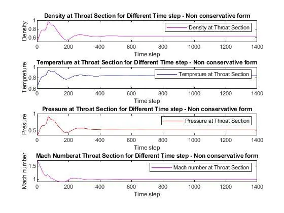
1.Primitive variables at throat section- non Conservative

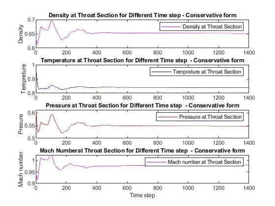
2. Primitive Variables at throat section - Conservative

3.Primitive variables along nozzle - Non Conservative

4. Primitive variables along nozzle - conservative

5. Mass flow rate -Nomn Conservative

6. Mass flow rate - Conservative

7. Mass flow rate - comparison

Results and Discussion

For primitive variables both techniques shows steady results after 500 time steps.We can observe from the above two graphs that , Velocity increases from inlet to outlet at the expense of pressure drop. Density and temperature drop from inlet to outlet as well .

Variation of Mass flow rate distribution inside the nozzle at different time steps during the time-marching process:we can see that conservative form seems to produce more consistent results when it comes to mass flow . In case of non-conservative graph, we note that results show huge variation near initial and final values .

From Conservative and Non-conservative perspective, we can oberve the following

a) Conservation form yields a better mass flow distribution or conservation of mass . We can observe this from the mass flow rate Vs Time step graph or Mass flow rate vs distance graph , where the results seems to be more consistent for conservative form . The conservative form tends to maintain a consisitent line , and has less deviation that non-conservative form .

b) Non-conservative form leads to a smaller residual . Non-conservative form does a better job in the sense that residual decay is an index of quality of numerical algorithm .

c) Non-conservative form seems to produce slightly more accurate results for primitive variables and conservative form seems to produce more accurate results for flux variables . The results in either case are satisfactory .

d) Conservative form requires more calculation time due to decoding of primitive variables to flux variables .