Week 5.1 - Mid term project - Solving the steady and unsteady 2D heat conduction problem
- Aim
Steady state analysis & Transient State Analysis
Solve the 2D heat conduction equation by using the point iterative techniques that were taught in the class. The Boundary conditions for the problem are as follows;
Top Boundary = 600 K
Bottom Boundary = 900 K
Left Boundary = 400 K
Right Boundary = 800 K
You will implement the following methods for solving implicit equations.
- Jacobi
- Gauss-seidel
- Successive over-relaxation
Your absolute error criteria is 1e-4
- Governing Equations
2D Heat conduction equation is (Transient equation)
Steady state :
We start with the mesh and describe the profile within the domain at discrete intervals. The spacing between the two discrete points in the x & y direction is dx and dy respectively.
- Steady State Condition
If omega=1, the SOR method simplifies to the Gauss-Seidel method. A theorem due to Kahan (1958) shows that SOR fails to converge if omega is outside the interval (0,2).
In general, it is not possible to compute in advance the value of omega that will maximize the rate of convergence of SOR. Frequently, some heuristic estimate is used, such as omega=2-O(h) where h is the mesh spacing of the discretization of the underlying physical domain.
Assume the value of omega = 1.25;
Matlab Code:
clear all
close all
clc
%assumptions
L=1;
%grid size
nx=10;
ny=10;
x=linspace(0,L,nx);
y=linspace(L,0,ny);
dx=L/(nx-1);
dy=L/(ny-1);
tol_err=1e-4;
%Boundary Conditions
T_T= 600;
T_B = 900;
T_L = 400;
T_R = 800;
%Matrix definition
T=275*ones(nx,ny);
T(1,:)=900;
T(end,:)=600;
T(:,1)=400;
T(:,end)=800;
%Boundary points rectangle
T(1,1)=(T_L+T_B)/2;
T(end,1)=(T_B+T_R)/2;
T(1,end)=(T_L+T_T)/2;
T(end,end)=(T_T+T_R)/2;
Told=T;

error=100;
%Iterative solver

k=2/dx^2 + 2/dy^2;
method=input('Enter the method of iteration    1.Jacobi, 2.Gauss-seidel, 3.SOR');
tic
if(method==1)
    iter_jaco=1;
    while(error>tol_err)

    for i=2:nx-1
        for j=2:ny-1
            term1=(Told(i-1,j)+Told(i+1,j))/(k*dx^2);
            term2=(Told(i,j-1)+Told(i,j+1))/(k*dy^2);
            T(i,j)=(term1+term2);
        end
    end
   error=max(max(abs(Told-T)));
    Told=T;
 iter_jaco= iter_jaco+1;
  figure(1)
        mesh(x,y,T);
       [A,B]=contourf(x,y,T);
       colorbar;
       colormap(jet);
        clabel(A,B);
        text=sprintf('Jacobi Iterations = %d',iter_jaco);
        xlabel('x');
        ylabel('y');
        title(text)
        pause(0.03)
    end
end
  if(method==2)
    iter_gauss=1;
    while(error>tol_err)

    for i=2:nx-1
        for j=2:ny-1
            term1=(T(i-1,j)+Told(i+1,j))/(k*dx^2);
            term2=(T(i,j-1)+Told(i,j+1))/(k*dy^2);
            T(i,j)=(term1+term2);
        end
    end
   error=max(max(abs(Told-T)));
    Told=T;
 iter_gauss= iter_gauss+1;
  figure(1)
        mesh(x,y,T);
       [A,B]=contourf(x,y,T);
       colorbar;
       colormap(jet);
        clabel(A,B);
        text=sprintf('Gauss-Seidal Iterations = %d',iter_gauss);
        xlabel('x');
        ylabel('y');
        title(text)
        pause(0.03)
    end
  end
  %define omega value is an assumption=1.25
alpha=1.25;
 if(method==3)
    iter_SOR=1;
    while(error>tol_err)

    for i=2:nx-1
        for j=2:ny-1
            term1=(T(i-1,j)+Told(i+1,j))/(k*dx^2);
            term2=(T(i,j-1)+Told(i,j+1))/(k*dy^2);
            T(i,j)=(1-alpha)*(Told(i,j))+alpha*(term1+term2);
        end
    end
   error=max(max(abs(Told-T)));
    Told=T;
 iter_SOR= iter_SOR+1;
  figure(1)
        mesh(x,y,T);
       [A,B]=contourf(x,y,T);
       colorbar;
       colormap(jet);
        clabel(A,B);
        text=sprintf('SOR Iterations = %d',iter_SOR);
       xlabel('x');
        ylabel('y');
        title(text)
        pause(0.03)
    end
end
toc
- Output
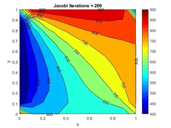
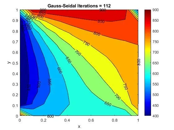
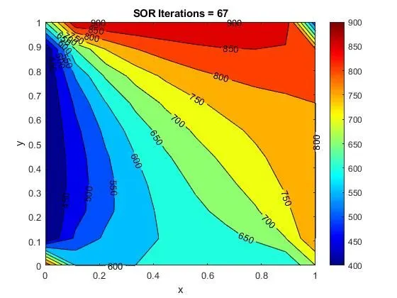
Found the values of Time Taken to complete the simulation and the amount of iterations.
The plots after simulation of Jacobi, guass-seidal and SOR is as follows
- Transient state heat conduction
For explicit method
For Implicit method
Matlab code for explicit method
clear all
close all
clc
%assumptions
L=1;
%grid size
nx=10;
ny=10;
x=linspace(0,L,nx);
y=linspace(L,0,ny);
dx=L/(nx-1);
dy=L/(ny-1);
%t=0.1, nt=t/dt;
dt=0.001;

tol_err=1e-4;
%Boundary Conditions
T_T= 600;
T_B = 900;
T_L = 400;
T_R = 800;
%Matrix definition
T=275*ones(nx,ny);
T(1,:)=900;
T(end,:)=600;
T(:,1)=400;
T(:,end)=800;
%Boundary points rectangle
T(1,1)=(T_L+T_B)/2;
T(end,1)=(T_B+T_R)/2;
T(1,end)=(T_L+T_T)/2;
T(end,end)=(T_T+T_R)/2;
Told=T;
error=100;
%diffusivity
alpha=1.4;
k1=alpha*dt/dx^2;
k2=alpha*dt/dy^2;
CFL=k1+k2;
unsteady_explicit_iter=1;
tic
for nt=1:1400
    while(error>tol_err)
        for i=2:nx-1
            for j=2:ny-1
                term1=Told(i-1,j)-2*Told(i,j)+Told(i+1,j);
                term2=Told(i,j-1)-2*Told(i,j)+Told(i,j+1);
                T(i,j)=Told(i,j)+k1*term1+k2*term2;
            end
        end
        error=max(max(abs(Told-T)));
        Told=T;
        unsteady_explicit_iter=unsteady_explicit_iter+1;

         figure(1)
        mesh(x,y,T);
       [A,B]=contourf(x,y,T);
       set(gca,'YDIR','reverse');
        colorbar
        colormap(jet)
        clabel(A,B);
        text=sprintf('Unsteady Explicit Iterations = %d',unsteady_explicit_iter);
        xlabel('x')
        ylabel('y')
        title(text)
        pause(0.03)
    end
end
toc
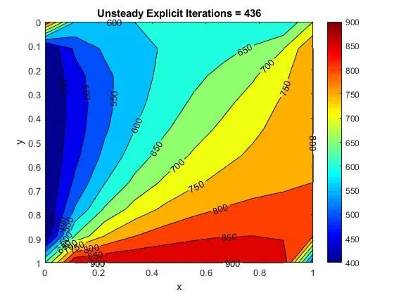
Output
Matlab code for Implicit Method
clear all
close all
clc
%assumptions
L=1;
%grid size
nx=10;
ny=10;
x=linspace(0,L,nx);
y=linspace(L,0,ny);
dx=L/(nx-1);
dy=L/(ny-1);
dt=0.001;
tol_err=1e-4;
%Boundary Conditions
T_T= 600;
T_B = 900;
T_L = 400;
T_R = 800;
%Matrix definition
T=275*ones(nx,ny);
T(1,:)=900;
T(end,:)=600;
T(:,1)=400;
T(:,end)=800;
%Boundary points rectangle
T(1,1)=(T_L+T_B)/2;
T(end,1)=(T_B+T_R)/2;
T(1,end)=(T_L+T_T)/2;
T(end,end)=(T_T+T_R)/2;
Told=T;
%diffusivity
alpha=1.4;
k1=alpha*dt/dx^2;
k2=alpha*dt/dy^2;
CFL=k1+k2;
unsteady_implicit_iter=1;
T_prev_dt=T;
omega = 1.25;
 iter=1;
method=input('Enter the method of iteration    1.Jacobi, 2.Gauss-seidel, 3.SOR');
tic
for time=1:1400
if (method==1)
     term1=(1+2*k1+2*k2)^(-1);
        term2=k1*term1;
        term3=k2*term1;
        error=1000;
    while(error>tol_err)
        for i=2:nx-1
                for j=2:ny-1

                    H=(Told(i-1,j)+Told(i+1,j));
                    V=(Told(i,j-1)+Told(i,j+1));
                    T(i,j) = (T_prev_dt(i,j)*term1)+(H*term2)+(V*term3);
                end
        end
           iter=iter+1;
           error=max(max(abs(Told-T)));
            Told=T;

    end
end
  if(method==2)
    term1=(1+2*k1+2*k2)^(-1);
        term2=k1*term1;
        term3=k2*term1;
        error=1000;
          while(error>tol_err)
               for i=2:nx-1
                for j=2:ny-1

                    H=(T(i-1,j)+Told(i+1,j));
                    V=(T(i,j-1)+Told(i,j+1));
                    T(i,j) = (T_prev_dt(i,j)*term1)+(H*term2)+(V*term3);
                end
               end

            error=max(max(abs(Told-T)));
            Told=T;
            iter=iter+1;
                end
  end
 if (method==3)


     term1=(1+2*k1+2*k2)^(-1);
        term2=k1*term1;
        term3=k2*term1;
        error=1000;
       while(error>tol_err)
        for i=2:nx-1
                for j=2:ny-1

                    H=(T(i-1,j)+Told(i+1,j));
                    V=(T(i,j-1)+Told(i,j+1));
                    T(i,j) = (1-omega)*Told(i,j)+omega*((T_prev_dt(i,j)*term1)+(H*term2)+(V*term3));
                end
         end

            error=max(max(abs(Told-T)));
            Told=T;
            iter=iter+1;

      end


 end
  T_prev_dt=T;
end
     toc
         figure(1)
        mesh(x,y,T);
       [A,B]=contourf(x,y,T);
       colorbar;
       colormap(jet);
        clabel(A,B);
        text=sprintf('Iterations = %d',iter);
        xlabel('x');
        ylabel('y');
        title(text)
        pause(0.03)
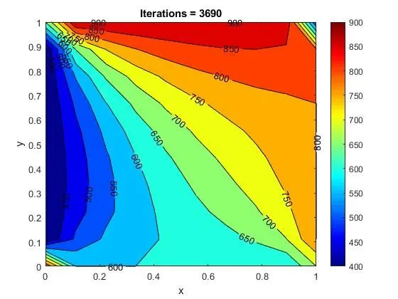
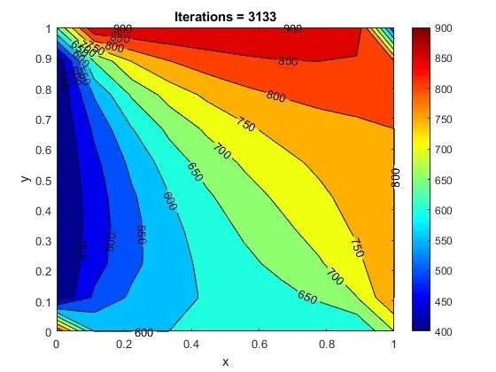
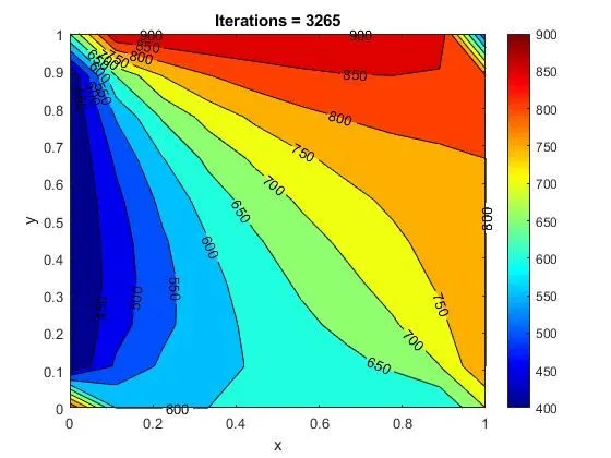
output
a. Jacobi
b.Gauss-seidal
c. SOR
Results and Discussion
- Steady state methods are converged easily as compared to transient. There are time loop included for implicit methods and it runs for a large number of iterations.
- Transient takes larger time for computation as it is a function of both time and position.
- The SOR provides us the answer with less number of iterations and takes less computation time.
CONCLUSION:
The 2D heat conduction equation solved.