Week 7 - Simulation of a 1D Super-sonic nozzle flow simulation using Macormack Method
%main program
clear all
close all
clc

% Initializing the domain

L = 3;                          % Length of Nozzle
nx = 31;                        %
x = linspace(0,L,nx)';          %
dx = x(2)-x(1);                 %
C = 0.5;                        % Courant Number
nt = 1400;                      % Time steps
gamma = 1.4;                    % Constant Value
A = 1 + 2.2*(x-1.5).^2;         % Nozzle area profile


% Computing the Flow Variable

% Non-Conservation Form
[rho1, V1, T1, p1, M1, m1, rho_t1, V_t1, p_t1, T_t1, M_t1, residual1] = nonconservative(x, dx, A, C, nt, gamma,nx);

% Conservation Form
[rho2, V2, T2, p2, M2, m2, rho_t2, V_t2, p_t2, T_t2, M_t2, residual2] = conservative(x, dx, A, C, nt, gamma);

% Steady-state distribution of primitive variables inside the nozzle
%for non conservative form
figure(1)
subplot(4,1,1)%mach number vs x
plot(x,M1,'r')
grid on;
ylim([0 4.5]);
yticks(0:1.5:4.5);
ylabel('Mach Number')
title('Flow parameter Non-Conservative Form)')
subplot(4,1,2)
plot(x,p1,'r')
grid on;
yticks(0:0.2:1);
ylabel('Pressure Ratio')
subplot(4,1,3)
plot(x,rho1,'r')
grid on; yticks(0:0.2:1);
ylabel('Density Ratio')
subplot(4,1,4)
plot(x,T1,'r')
grid on; ylim([0 1]); yticks(0:0.2:1);
ylabel('Temperature Ratio')
xlabel('X/L')


figure(2)
subplot(4,1,1)
plot(x,M2)
grid on;
ylim([0 4.5]);
yticks(0:1.5:4.5);
ylabel('Mach Number')
title('Flow parameters Conservative Form)')
subplot(4,1,2)
plot(x,p2)
grid on;
yticks(0:0.2:1);
ylabel('Pressure Ratio')
subplot(4,1,3)
plot(x,rho2)
grid on;
yticks(0:0.2:1);
ylabel('Density Ratio')
subplot(4,1,4)
plot(x,T2)
grid on;
ylim([0 1]);
yticks(0:0.2:1);
ylabel('Temperature Ratio')
xlabel('X/L')


% Time-wise variation of the primitive variables
figure(3)
subplot(4,1,1)
plot(1:nt,rho_t1)
hold on
plot(1:nt,rho_t2)
grid on; ylim([0 1]); yticks(0:0.2:1);
ylabel('rho/rho_0')
title('Flow Parameter variation with time at the Nozzle Throat');
legend('Non-conservative','Conservative');
subplot(4,1,2)
plot(1:nt,T_t1)
hold on
plot(1:nt,T_t2)
grid on; yticks(0:0.2:1);
ylabel('T/T_0')
legend('Non-conservative','Conservative');
subplot(4,1,3)
plot(1:nt,p_t1)
hold on
plot(1:nt,p_t2)
grid on; yticks(0:0.2:1);
ylabel('p/p_0')
legend('Non-conservative','Conservative')
subplot(4,1,4)
plot(1:nt,M_t1)
hold on
plot(1:nt,M_t2)
grid on; yticks(0:0.2:2);
ylabel('Mach No.')
xlabel('Time Steps')
legend('Non-conservative','Conservative')


figure(4)
subplot(2,1,1)
plot(1:nt,residual1)
grid on
xlabel('Time Steps')
ylabel('Residuals')
legend('|drho/dt|_{av}','|dV/dt|_{av}','|dT/dt|_{av}')
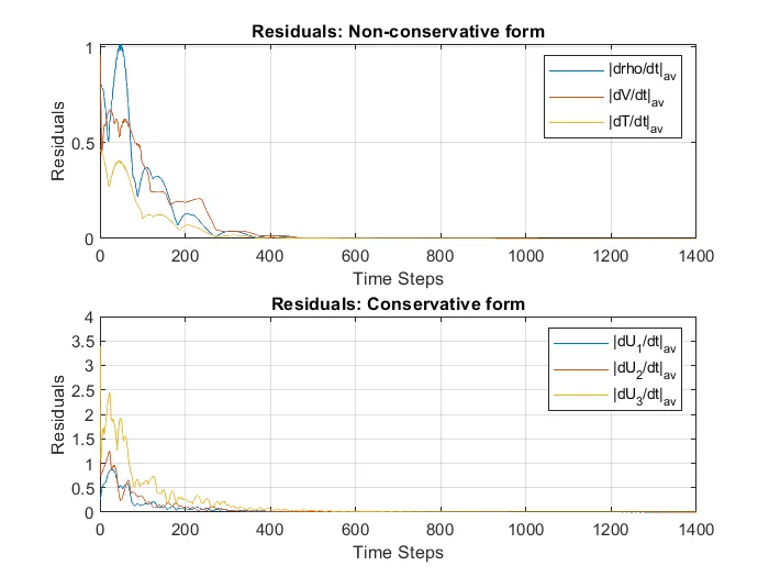
title('Residuals: Non-conservative form')
subplot(2,1,2)
plot(1:nt,residual2)
grid on
xlabel('Time Steps')
ylabel('Residuals'); yticks(0:0.5:4);
legend('|dU_1/dt|_{av}','|dU_2/dt|_{av}','|dU_3/dt|_{av}')
title('Residuals: Conservative form')

% Variation of Mass flow rate distribution inside the nozzle at different
% time steps during the time-marching process for Non-Conservation Form
figure(5)
hold on; grid on;
plot(x,m1(50,:),'-x')
plot(x,m1(100,:),'-d')
plot(x,m1(150,:),'-s')
plot(x,m1(200,:),'-*')
plot(x,m1(700,:),'-o')
xlabel('X/L')
ylabel('rhoAV/rho_0A_0V_0')
legend('t = 50/t','t = 100/t','t = 150/t','t = 200/t','t = 700/t')
title('Variation of Mass Flow Rate - Non-conservative form')

% Variation of Mass flow rate distribution inside the nozzle at different
% time steps during the time-marching process for Conservation Form
figure(6)
hold on; grid on;
plot(x,m2(100,:),'-x')
plot(x,m2(150,:),'-d')
plot(x,m2(200,:),'-*')
plot(x,m2(700,:),'-o')
xlabel('X/L')
ylabel('rhoAV/rho_0A_0V_0')
legend('t = 100/t','t = 150/t','t = 200/t','t = 700/t')
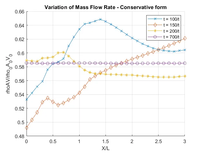
title('Variation of Mass Flow Rate - Conservative form')


%Normalized mass flow rate distributions for Conservation & Non-Conservatio Form

figure(7)
hold on; grid on;
plot(x,m1(end,:),'LineWidth',3)
plot(x,m2(end,:),'LineWidth',3)
plot(x,0.579*ones(length(x),1),'--k')
xlabel('X/L')
ylabel('rhoAV/rho_0A_0V_0')
legend('Non-Conservative','Conservative','Exact')
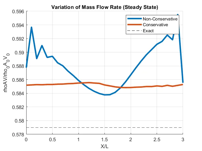
title('Variation of Mass Flow Rate (Steady State)')
% Solver for Non-Conservative Form of Governing Equation
function [rho, V, T, p, M, m, rho_t, V_t, p_t, T_t, M_t, residual] = nonconservative(x, dx, A, C, nt, gamma,nx)

% Initial conditions
rho_0 = 1 - 0.3146*x;
T_0 = 1 - 0.2314*x;
V_0 = (0.1 + 1.09*x).*T_0.^0.5;

throat = find(A==1);
rho = rho_0;
T = T_0;
V = V_0;

m = zeros(nt,length(x));
rho_t = zeros(nt,1);
T_t = rho_t;
V_t = T_t;
p_t = V_t;
M_t = p_t;

residual = zeros(nt,3);

%-------Macromack Method----%
% ----Non-Conservation Equation------------%

% Outer time loop
for k=1:nt
    rho_old = rho;
    T_old = T;
    V_old = V;
    dt = min(C*dx./(T.^0.5 + V));

% Predictor loop
    for i=2:nx-1
        % Equation Simplified - Forward Difference
        dVdx = (V(i+1) - V(i))/dx;
        dlogAdx = (log(A(i+1))-log(A(i)))/dx;
        drhodx = (rho(i+1) - rho(i))/dx;
        dTdx = (T(i+1) - T(i))/dx;

        % Continuity, Momentum & Energy Equations
        drhodt_p(i) = -rho(i)*dVdx - rho(i)*V(i)*dlogAdx - V(i)*drhodx;
        dVdt_p(i) = -V(i)*dVdx - (1/gamma)*(dTdx + (T(i)/rho(i))*drhodx);
        dTdt_p(i) = -V(i)*dTdx - (gamma-1)*T(i)*(dVdx + V(i)*dlogAdx);

        % Intermediate Solution Update
        rho(i) = rho(i) + drhodt_p(i)*dt;
        V(i) = V(i) + dVdt_p(i)*dt;
        T(i) = T(i) + dTdt_p(i)*dt;
    end

    % Corrector loop
    for i=2:nx-1
        % Equation Simplified - Backward Difference
        dVdx = (V(i) - V(i-1))/dx;
        dlogAdx = (log(A(i))-log(A(i-1)))/dx;
        drhodx = (rho(i) - rho(i-1))/dx;
        dTdx = (T(i) - T(i-1))/dx;

        % Continuity, Momentum & Energy Equations
        drhodt_c(i) = -rho(i)*dVdx - rho(i)*V(i)*dlogAdx - V(i)*drhodx;
        dVdt_c(i) = -V(i)*dVdx - (1/gamma)*(dTdx + (T(i)/rho(i))*drhodx);
        dTdt_c(i) = -V(i)*dTdx - (gamma-1)*T(i)*(dVdx + V(i)*dlogAdx);
    end

    % Compute Average Time Derivative
    drhodt = 0.5*(drhodt_p + drhodt_c);
    dVdt = 0.5*(dVdt_p + dVdt_c);
    dTdt = 0.5*(dTdt_p + dTdt_c);

    residual(k,1) = max(abs(drhodt));
    residual(k,2) = max(abs(dVdt));
    residual(k,3) = max(abs(dTdt));

    % Final solution update
    for i=2:nx-1
        rho(i) = rho_old(i) + drhodt(i)*dt;
        V(i) = V_old(i) + dVdt(i)*dt;
        T(i) = T_old(i) + dTdt(i)*dt;
    end

    % Applying Boundary Conditions
    % Inlet BCs
    V(1) = 2*V(2)-V(3);

    % Outlet BCs
    rho(end) = 2*rho(end-1)-rho(end-2);
    V(end) = 2*V(end-1)-V(end-2);
    T(end) = 2*T(end-1)-T(end-2);


    % Equating Primitive Variables
    M = V./(T.^0.5);%mach no
    p = rho.*T;% pressure ratio
    m(k,:) = rho.*A.*V;%mass flow rate
    rho_t(k) = rho(throat);%desity ratio saved for all time interval at throat
    V_t(k) = V(throat); % veloty ratio  saved for all time intrerval at throat
    T_t(k) = T(throat);%temp ratio saved for all time intrerval at throat
    p_t(k) = p(throat);%pressure ratio saved for all time intrerval at throat
    M_t(k) = M(throat);%mach no saved for all time intrerval at throat
end
% End of Non-Coservation Function
end
% Solver for Conservative Form of Governing Equation
function [rho, V, T, p, M, m, rho_t, V_t, p_t, T_t, M_t, residual] = conservative(x, dx, A, C, nt, gamma)

% Initial conditions
rho_0 = zeros(length(x),1);
T_0 = rho_0;
V_0 = T_0;

for i=1:length(x)
    if x(i)>=0 && x(i)<0.5
        rho_0(i) = 1;
        T_0(i) = 1;
    elseif x(i)>=0.5 && x(i)<1.5
        rho_0(i) = 1 - 0.366*(x(i)-0.5);
        T_0(i) = 1 - 0.167*(x(i)-0.5);
    elseif x(i)>=1.5 && x(i)<=3
        rho_0(i) = 0.634 - 0.3879*(x(i)-1.5);
        T_0(i) = 0.833 - 0.3507*(x(i)-1.5);
    end
    V_0(i) = 0.59/(rho_0(i)*A(i));
end

throat = find(A==1);%to find the position of throat
rho = rho_0;
T = T_0;
V = V_0;
m = zeros(nt,length(x));

% U!,U2 and U3 calculated
U1 = rho.*A;
U2 = rho.*A.*V;
U3 = rho.*(T./(gamma-1) + 0.5*gamma*V.^2).*A;

rho_t = zeros(nt,1);
T_t = rho_t;
V_t = T_t;
p_t = V_t;
M_t = p_t;

residual = zeros(nt,3);

%-------Macromack Method----%
% ----Conservation Equation------------%

% Outer Time Loop
for k=1:nt
    %saving old data
    U1_old = U1;
    U2_old = U2;
    U3_old = U3;
%     finding min time interval to convege fast
    dt = min(C*dx./(T.^0.5 + V));

    F1 = U2;
    F2 = (U2.^2)./U1+((gamma-1)/gamma)*(U3 - 0.5*gamma*(U2.^2)./U1);
    F3 = gamma*U2.*U3./U1 - 0.5*gamma*(gamma-1)*(U2.^3)./(U1.^2);

    % Predictor loop
    for i=2:length(x)-1
        % Equation Simplified - Forward Difference
        dF1dx = (F1(i+1) - F1(i))/dx;
        dF2dx = (F2(i+1) - F2(i))/dx;
        dF3dx = (F3(i+1) - F3(i))/dx;
        dAdx = (A(i+1) - A(i))/dx;
        J2 = (1/gamma)*rho(i)*T(i)*dAdx;

        % Continuity, Momentum & Energy Equations
        dU1dt_p(i) = -dF1dx;
        dU2dt_p(i) = -dF2dx + J2;
        dU3dt_p(i) = -dF3dx;

        % Intermediate Solution Update
        U1(i) = U1(i) + dU1dt_p(i)*dt;
        U2(i) = U2(i) + dU2dt_p(i)*dt;
        U3(i) = U3(i) + dU3dt_p(i)*dt;
    end

    rho = U1./A;
    V = U2./U1;
    T = (gamma-1)*((U3./U1) - 0.5*gamma*V.^2);

    F1 = U2;
    F2 = (U2.^2)./U1+((gamma-1)/gamma)*(U3 - 0.5*gamma*(U2.^2)./U1);
    F3 = gamma*U2.*U3./U1 - 0.5*gamma*(gamma-1)*(U2.^3)./(U1.^2);

    % Corrector loop
    for i=2:length(x)-1
        % Equation Simplified - Backward Difference
        dF1dx = (F1(i) - F1(i-1))/dx;
        dF2dx = (F2(i) - F2(i-1))/dx;
        dF3dx = (F3(i) - F3(i-1))/dx;
        dAdx = (A(i) - A(i-1))/dx;
        J2 = (1/gamma)*rho(i)*T(i)*dAdx;

        % Continuity, Momentum & Energy Equations
        dU1dt_c(i) = -dF1dx;
        dU2dt_c(i) = -dF2dx + J2;
        dU3dt_c(i) = -dF3dx;
    end

    % Compute Average Time Derivative
    dU1dt = 0.5*(dU1dt_p + dU1dt_c);
    dU2dt = 0.5*(dU2dt_p + dU2dt_c);
    dU3dt = 0.5*(dU3dt_p + dU3dt_c);

    residual(k,1) = max(abs(dU1dt));
    residual(k,2) = max(abs(dU2dt));
    residual(k,3) = max(abs(dU3dt));

        % Final solution update
    for i=2:length(x)-1
        U1(i) = U1_old(i) + dU1dt(i)*dt;
        U2(i) = U2_old(i) + dU2dt(i)*dt;
        U3(i) = U3_old(i) + dU3dt(i)*dt;
    end

   % Boundary COnditions
   % Inlet BCs
   U1(1) = rho(1)*A(1);
   U2(1) = 2*U2(2) - U2(3);
   U3(1) = U1(1)*((T(1)/(gamma-1)) + 0.5*gamma*V(1)^2);

   % Outlet BCs
   U1(end) = 2*U1(end-1) - U1(end-2);
   U2(end) = 2*U2(end-1) - U2(end-2);
   U3(end) = 2*U3(end-1) - U3(end-2);

   % Equating Primitive Variables
    rho = U1./A;
    V = U2./U1;
    T = (gamma-1)*((U3./U1) - 0.5*gamma*V.^2);
    M = V./(T.^0.5);%mach no
    p = rho.*T;% pressure ratio

    m(k,:) = rho.*A.*V;%mass flow rate
    rho_t(k) = rho(throat); %desity ratio saved for all time interval at throat
    V_t(k) = V(throat); % veloty ratio  saved for all time intrerval at throat
    T_t(k) = T(throat);%temp ratio saved for all time intrerval at throat
    p_t(k) = p(throat); %pressure ratio saved for all time intrerval at throat
    M_t(k) = M(throat);%mach no saved for all time intrerval at throat
end
% End Function
end
explaination:-
Aim:-
simulate the isentropic flow through a quasi 1D subsonic-supersonic nozzle for both conservation and non conservation form and solve using MacCormack's technique
governing eqn
Continuity, Momentum & Energy Equations
`drho/dt=-rho*dv/dx-rho*v*dlnA/dx-v*drho/dx`
`dv/dt=v*dv/dx-1/gamma*(dt/dx+t/rho*drho/dx)`
`dv/dt=v*dv/dx-1/gamma*(dt/dx+t/rho*drho/dx)``dT/dx=v*dT/dx-(gamma-1)*T*(dv/dx+v*dlnA/dx)`
Intermediate Solution Update
`rho = rho+ drho/dt*dt`
`V = V+ dV/dt*dt`
`T= T+ dT/dt*dt`
`M=v/T^0.5`
`p=rho*T`
`m=rho*v*A`
`u1=rho*A`
`u2=rho*A*v`
`U3 = rho*(T/(gamma-1) + 0.5*gamma*V.^2)*A`
F1 = U2
`F_3 = gamma*U_2*U_3/U_1 - 0.5*gamma*(gamma-1)*(U_2^3)/(U_1.^2);`
`F_2 = (U_2^2)/U_1+((gamma-1)/gamma)*(U_3 - 0.5*gamma*(U_2^2)./U_1);`
`dF_1/dx = (F_1(i+1) - F_1(i))/dx`Forward Difference
`dF_1/dx = (F_1(i) - F_1(i-1))/dx`Backward Difference
Intermediate Solution Update
`U1 = U1 + dU1dt*dt;`
``U2= U2 + dU2dt*dt`
``U3 = U3 + dU3dt*dt;``
Aim:-
simulate the isentropic flow through a quasi 1D subsonic-supersonic nozzle for both conservation and non conservation form and solve using MacCormack's technique
governing eqn
`rho = rho+ drho/dt_p*dt`
`V = V+ dV/dt_p*dt`
`T= T+ dT/dt_p*dt`
rho-disity ratio
T temprature ratio
v-velocit ratio
A area
M=mach no
m mass flow rate
Body of content:-
1.
non consertvation function define
first intiala codtion are given
now entered into time loop for nt times
old premitive variable are saved
then using cfl fromula minimum dt is found which will help to converge eqn fast
enter into space loop
Predictor loop
dv/dx,drho/dx,dT/dx and dlnA/dx is calculated using Forward Difference method
the above value is used to calculate drho/dt,dv/dt and dT/dt using governing eqn ie Continuity, Momentum & Energy Equations
the Intermediate Solution Update
using governing eqn
Corrector loop
dv/dx,drho/dx,dT/dx and dlnA/dx is calculated using Forward Difference method
the above value is used to calculate drho/dt,dv/dt and dT/dt using governing eqn ie Continuity, Momentum & Energy Equations
Compute Average Time Derivative
drho/dt,dv/dt and dT/dt is calclatd by taking avrg of drho/dt,dv/dt and dT/dt of both predictor and corrector loop
Final solution update
rho, v and T is calculted using governing eqn
boundary condtion
inlet and outlet boundary condition is calcuating extarapolation the avalble data
new values updated
2.
consertvation function define
first intiala codtion are given
and u1,u2 and u3 is calctaled ising governing eqn
now entered into time loop for nt times
old premitive variable are saved
then using cfl fromula minimum dt is found which will help to converge eqn fast
f1,f2,f3 abd j2 is calcualted using governing eqn
enter into space loop
Predictor loop
now simmilar Forward Difference method is used to calculate df1/dx,df2/dx and df3/dx
then using governing eqn ie Continuity, Momentum & Energy Equations
du1/dt,du2/dt and du3/dt is calculated
the Intermediate Solution Update
using governing eqn
update the old u1,u2 and u3 with new value
Corrector loop
now simmilar Backward Difference method is used to calculate df1/dx,df2/dx and df3/dx
then using governing eqn ie Continuity, Momentum & Energy Equations
du1/dt,du2/dt and du3/dt is calculated
Compute Average Time Derivative
now take the avrg du1/dt,du2/dt and du3/dt of both predictor and corrector loop
Final solution update
boundary condtion
inlet and outlet boundary condition is calcuating extarapolation the avalble data
from above date primitive variables are calculated
Main file
here intial data is given like L,x,nx,A,c and gamma
then both the function called
plots
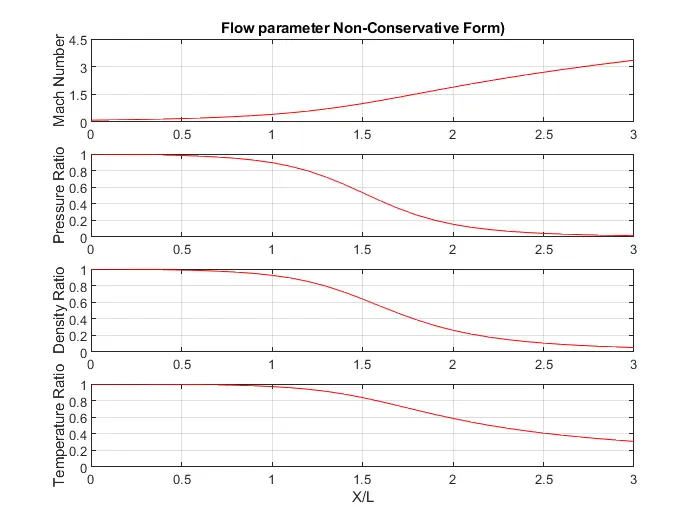
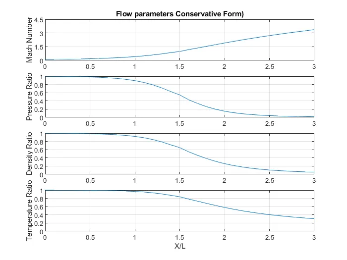
figure (1&2)
Flow parameter Non-Conservative Form and Conservative Form
mach no is increasing along the x from sub sonic flow to super sonic flow
pressure ratio,velocity ratio and temparature ratio is gradully dropping along the x
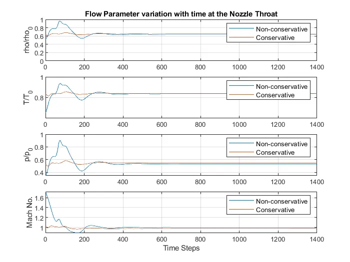
figure(3)
Flow Parameter variation with time at the Nozzle Throat
from plot its seen that the conservation form is more stable and converge fast than the non conservation form
figure(4)
Residuals
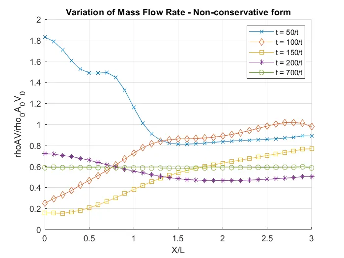
figure(5)
Variation of Mass Flow Rate - Non-conservative form
fuigure(6)
Variation of Mass Flow Rate - conservative form
figure(7)
Variation of Mass Flow Rate