Week 7 - Simulation of a 1D Super-sonic nozzle flow simulation using Macormack Method

Aim: Simulation of a 1D Super-sonic nozzle flow simulation using Macormack Method.

In this challenge you are going to simulate the isentropic flow through a quasi 1D subsonic-supersonic nozzle. You will derive both the conservation and non-conservation forms of the governing equations and sovle them using the MacCormack's technique. You need to determine the steady-state temperature distribution for the flow-field variables and investigate the difference between the two forms of governing equations by comparing their solutions.

we need to show the following plots inside your report
1. Steady-state distribution of primitive variables inside the nozzle
2. Time-wise variation of the primitive variables
3. Variation of Mass flow rate distribution inside the nozzle at different time steps during the time-marching process
4. Comparison of Normalized mass flow rate distributions of both forms

Theory:

Introduction:Direct numerical stimulation of fluid flow through nozzle has always been a challenging problem and an area of immense interest for modern engineers. Converging-Diverging nozzle has been extensively used in a wide range of Industrial
applications ranging from steam turbines to rocket engine nozzles.

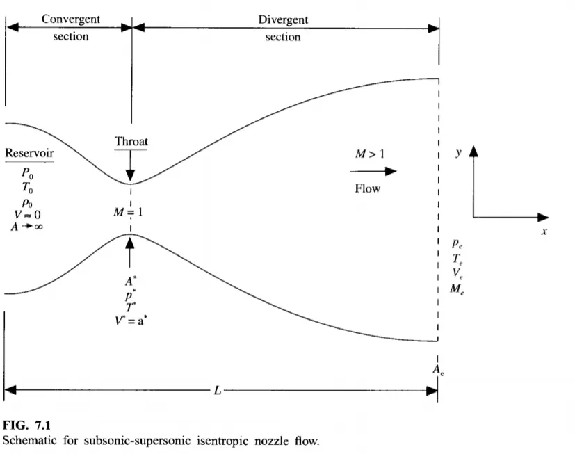
The condition for operation so that the nozzle produces supersonic flow is that the Mach number at throat should be equal to one. This condition is known as choked flow. As the fluid expands further in the diverging section, the fluid flow increases to supersonic velocities.(Mach Number>1).If the choke condition is not met, the nozzle simply acts as a Venturi tube and would produce subsonic flow even at the outlet. This paper uses an explicit finite difference scheme for numerical solution of fluid flow. This scheme is fully explicit and second order accurate in both time and space.

MACH NUMBER- The Mach number is a dimensionless quantity representing the ratio of flow velocity past a boundary to the local speed of sound.

M=v/√T

where:

M is the Mach number

v is the velocity of the flow

T is the speed of sound

Maccormack method:

To discretize the numerical solution we use the technique called the Macormack method. The MacCormack method is a variation of the two-step Lax-Wendroff Scheme but is much simpler in the application.

The application of the Maccormack method proceeds in two steps; a predictor step which is followed by a corrector step.

• Predictor step: In the predictor step, a "provisional" value of at time level (denoted by ) is estimated obtained by replacing the spatial and temporal derivatives in the previous first-order equation using Forward Difference Scheme. is used for Timestep.
• Corrector step: In the corrector step, the predicted value is corrected according to the equation. Note that the corrector step uses the Backward Difference Scheme for spatial derivative. The time-step used in the corrector step is in contrast to the used in the predictor step.

For non-conservation form.

Predictor method.

we will be applying the forward differencing to the right-hand side spatial derivatives in the predictor method.

The continuity equation for the non-conservative form for the predictor method.

(dρ/dt)p=(−ρ[(⋅v(i+1)−v(i)]/dx)−(ρ⋅v⋅[log(a(i+1))−log(a(i))]/dx)−(v⋅[ρ(i+1)−ρ(i)]/dx)

The momentum equation for the non-conservative form for the predictor method.

(dv/dt)p=−v⋅([v(i+1)−v(i)]/dx)−(1/γ)⋅([t(i+1)−t(i)]/dx+(t/ρ)⋅[ρ(i+1)−ρ(i)]/dx)

The energy equation for the non-conservative form for the predictor method.

(dT/dt)p=−v⋅[t(i+1)−t(i)]/dx−(γ−1)⋅t⋅[(v(i+1)−v(i)]/dx+v⋅[log(a(i+1))−log(a(i))]/dx)

Corrector method.

In the corrector method rearward differencing is applied to the right-hand side spatial derivatives.

The continuity equation for the non-conservative form for the corrector method.

(dρ/dt)c=(−ρ[(⋅v(i)−v(i−1)]/dx)−(ρ⋅v⋅[log(a(i))−log(a(i−1))]/dx)−(v⋅[ρ(i)−ρ(i−1)]/dx)

The continuity equation for the non-conservative form for the corrector method.

(dv/dt)c=−v⋅[(v(i)−v(i−1)]/dx)−(1/γ)⋅[(t(i)−t(i−1)]/dx+(t/ρ)⋅[ρ(i)−ρ(i−1)]/dx)

The energy equation for the non-conservative form for the corrector method.

(dT/dt)c=−v⋅[t(i)−t(i−1)]/dx−(γ−1)⋅t⋅[(v(i)−v(i−1)]/dx+v⋅[log(a(i))−log(a(i−1))]/dx)

The average time derivatives.

by adding both the conservative and non-conservative equations and taking the average of them we get, density, velocity, and temperature terms as,

(dρ/dt)av=[(dρ/dt)p+(dρ/dt)c]/2

(dv/dt)av=[(dv/dt)p+(dv/dt)c]/2

(dT/dt)av=[(dT/dt)p+(dT/dt)c]2

For conservation form.

Predictor method.

The continuity equation for the conservative form for the predictor method.

(dU1/dt)p=−[F1(i+1)−F1(i)]/dx

The momentum equation for the conservative form for the predictor method.

(dU2/dt)p=−[(F2(j+1)−F2(j)]/dx)+J2

where,

source term,

J2=(1/γ)⋅ρ⋅T⋅[a(i+1)−a(i)]/dx

The energy equation for the conservative form for the predictor method.

(dU3/dt)p=−[F3(i+1)−F3(i)]/dx

Corrector method

The continuity equation for the conservative form for the corrector method.

(dU1/dt)c=−[F1(i)−F1(i−1)]/dx

The momentum equation for the conservative form for the corrector method.

(dU2/dt)c=−([F2(i)−F2(i−1)]/dx)+J2(i)

where,

source term,

JJ2=(1/γ)⋅ρ⋅T⋅[a(i)−a(i−1)]/dx

The energy equation for the conservative form for the corrector method.

(dU3/dt)c=−[F3(i)−F3(i−1)]/dx

Flux vectors,

F1=U2

F2=(U2^2/U1)+γ−1/γ⋅(U3−(γ/2)⋅(U2^2/U1))

F3=((γ⋅U2⋅U3/U1)−γ⋅(γ−1/2)⋅(U2^3/U1^2))

solution vectors,

U1=ρ⋅a

U2=ρ⋅a⋅v

U3=ρ⋅(T/γ−1+(γ/2)⋅v^2)⋅a

where,

rho is the density

a is the area through the nozzle

v is the local velocity

T is the temperature

γ">γ is the ratio of specific heats

Average time derivatives,

(dU1/dt)av=[(dU1/dt)p+(dU1/dt)c]/2

(dU2/dt)av=[(dU2/dt)p+(dU2/dt)c]/2

(dU3/dt)av=[(dU3/dt)p+(dU3/dt)c]/2

Initial conditions(at the time =0);

Depending on the values of x-node we are setting up the values for rho,V and T.

rho=1-0.3146x.

V=1-0.2314x

T=(0.1=1.09x)T^0.5.

Nozzle shape:

For area(A),we are going to set up a profile.

A=1+2.2(x-1.5)^2 0<x<3.

Mach number:

M=V/√T.

Calculation of time step:

For both non-conservative and conservative form of governing equation we are going to take time step.

Δt=c(Δx/a+v)

where C=courant number

V=local flow velocity

a=locl speed of sound.

for an eplicit numerical solution to be stable C<1 ,here we are taking C=0.5.

Equation given above is the CFL criterion for a one dimensional flow along with C<1 it simply states that delta t must be less than or at best equal to the time taken by a sound wave to move from one grid point to the next.

Deltax is the same throughout the flow,but both V' and a are variables.hence at a given grid points ata given time step.

(Δt^t)i=C[Δx/(a^t)i+(V^t)i]

And at an adjacent grid point:

(Δt^t)i+1=C[Δx/(a^t)i+1+(V^t)i+1]

Boundary conditions:

subsonic inflow boundary (at node1 )

We must allow one varibale to float,we choose the velocity V because on a physical basis we know that the mass flow through the nozzle must be allowed to adjust to the proper steady state and allowing V to float makes the complete sense as part of this adjustment

V1=2V2-V3

Density and temperature are fixed (independent of time)

rho1=1 and T1=1

Supersonic outflow boundary(at node N)

we must allow all flow field variables to float.

V(n)=2⋅V(n−1)−V(n−2)

ρ(n)=2⋅ρ(n−1)−ρ(n−2)

T(n)=2⋅T(n−1)−T(n−2)

Conservative form of governing equations:

Governing equations for quasi-one-dimensional flow in conservative form is given by

Continuity:

conservtaive form

[∂(ρ'A')]/∂t'+[∂(ρ'A'V')]∂x'=0

Momentum:

conservative form:

[∂(ρ'A'V')]/∂t'+[∂[ρ'A'(V')^2+1/γ.ρ'A']/∂x'=1/γρ'∂A/'∂x

Energy:

conservtaive form:

[∂[ρ'e'γ−1+γ2(V')2A']]/∂t'+[∂[ρ'e'γ−1+γ2(V')2)V'A'+ρ'A'V']/∂x'=0

The governing equations fro quasi one dimensional flow can be expressed in a more genric form by defining the elements as the solution vector U the flux vector F and the source term J as follows.

U1=ρ'⋅A'

U2=ρ′⋅A′⋅V′

U3=ρ′[e'/γ-1+γ/2(V')^2]A′

F1=ρ′⋅A′⋅V′

F2=ρ′⋅A′⋅(V′)^2+1/γ⋅ρ′⋅A′

F3=ρ′(e′/γ-1+γ/2(V′)^2)A′V′+P′A′V′

J2=(1/γ)P′.∂A′/∂x′

with these elements governing equations can be written as;

Continuity:

∂U1/∂t'=−∂F1/∂x'

Momentum:

∂U2/∂t'=−∂F2/∂x'+J2

Energy:

∂U3/∂t'=−∂F3/∂x'

In the conservative form of governing equations the dependent variables to obtain the primitive variables(rho,V,P,T etc...) we must decode the elements U1,U2,U3 as follows.

ρ'=U1/A'

V'=U2/U1

T'=e'−(γ−1)U3/U2−γ/2(V')^2

P'=ρ'⋅T'

Therefore after we obtain U1,U2 and U3 at each time step from the numerical solution of equations we can immediately calculate the corresponding primitive variables at each time step rho',V',T' and P'.

Pure from of flux vector is given by;

F1=U2

F2=U2^2/U1+γ−1/γ[U3−(γ/2)U2^2/U1^2]

F3=γ(U2U3/U1)−γ(γ−1/2)(U2^3/U1^2)

J2=(γ−1/γ)(U3−(γ/2)(U2^2/U1)(∂(lnA')/∂x')

This is the pure form of governing equation in conservative form.

Initial conditions:

for 0<x'0.5: rho'=1.0 and T' =1.0

for 0.5<1.5: rho'=1.0-0.366(x'-0.5) and T'=1.0-0.167(x'-0.5)

for 1.5<x'<3.0: rho'=0.634-0.3879(x'-1.5) and T'=0.833-0.3507(x'-1.5) .

for the initial condition only,lets assume a constant mass flow through the nozzle and calculate V as,

V'=U2/ρ'A'=0.59/ρ'A'

The value of 0.59 is chosen for U2 because it is the closest to the exact analytical value of the steady state mass flow (i.e)=0.579.

Boundary conditions:

Subsonic inflow boundary (at node 1)

Two properties are held fixed and one is allowed to float rho and T are fixed at inflow boundary both equal to 1 and allowing V to float.

(U11)i=1=ρ'A'i=1

(U2)i=2=2(U2)i=2−(U2)i=3

(U3)i=1=ρ'[(e'/γ−1)+γ/2V'2]A'

Supersonic outflow boundary(at node N)

All properties are allowed to float:

(U1)n=2(U1)n−1−(U1)n−1

(U2)n=2(U2)n−1−(U2)n−1

(U3)n=2(U3)n−1−(U3)n−1

PROGRAM LOGIC.

• Let's start with the clear commands clear all, close all, clc
• And then assigning the values that is for n, x, dx, gamma as an input parameters.
• calculating the initial profile for both the conservative and non-conservative forms that is density, temperature, and velocity values and also calculating the area and assigning the number of time steps.
• and we have created the functions to computing for both the conservative and non-conservative forms and plottings will also be done within the functions so in the main program, we are just going to call those functios to get the results.
• and only one plot has to be made in the main program that is to compare both the convservative and non-conservative mass flow rates in a single graph that can be done.

CODE.

Main program :-

clear all
close all
clc

% inputs
n=31;
x=linspace(0,3,n);
% z=linspace(0,1400,n);
dx=x(2)-x(1);
gamma=1.4;
throat=(n-1)/2;

% calculate the initial profile
for m=1:n

if (x(m)>=0&&x(m)<=0.5)
rho_c(m)=1;
t_c(m)=1;
elseif (x(m)>=0.5&&x(m)<=1.5)

rho_c(m)=1-0.366*(x(m)-0.5);
t_c(m)=1-0.167*(x(m)-0.5);

elseif (x(m)>=1.5&&x(m)<=3.5)

rho_c(m)=0.634-0.3879*(x(m)-1.5);
t_c(m)=0.833-0.3507*(x(m)-1.5);

end
end

% area
a=1+2.2*(x-1.5).^2;

% time step
nt=1400;

% conservation form
[rho,v,p,mass_flow_rate,M_c]=one_d_conservation_form_func(n,x,dx,gamma,throat,rho_c,t_c);

% non conservation form
[rho_tr,p_tr,t_tr,m,p_nc,M_nc,t_nc]=one_d_supersonic_nozzle_flow_func(n,x,dx,gamma,throat);

figure(8)
plot(x,mass_flow_rate,'r')
hold on
plot(x,m,'b')
plot(x,0.579,'p')
legend('conservative form','Non conservative form')
xlabel('No of nodes')
ylabel('Mass flow rate')
title(' Comparison of Normalized mass flow rate distributions of both forms')

Function for computing the values of the non-conservative form.

• The function has created to calculate the values of Mass flow rate, Pressure, Mach number, Density, velocity, Temperature, Density at throat, velocity at throat, Temperature at throat, Mass flow rate at throat, Pressure at throat, Mach number at throat by the known equations for all the grid points.
• For this initial boundary conditions are taken for Density, Temperature & Velocity and profiles for calculating area & throat.
• Now Outer Time loop will compute for for loop to calculate all the grid points for various formulas inside the loop.
• MacCarmack technique is used to solve the numerical solution of governing equations such as Continuity, Momentum & Energy Equation.
• The technique implies two methods for solving namely Predictor method followed by Corrector method.
• Predictor & Corrector method are assigned within the for loop individually for calculating values.
• The calculated values are averaged in the next step and updating the solution with old values.
• Boundary Conditions are applied within the for loop and subsequently used for calculating the Mass Flow Rate, Mach Number & Pressure and also calculating the values throat section.
• And also the plottings will be done within the functions only so that we can easily call the function and get the results.
• The plots for the variation of primitive variables at the steady state and at the throat will be plotted.
• Plot for Distance through the nozzle & Mass Flow Rate for differrent Timesteps has done within the function.
• Here we are going to end the function.

function [rho_tr,p_tr,t_tr,m,p_nc,M_nc,t_nc]=one_d_supersonic_nozzle_flow_func(n,x,dx,gamma,throat)

% calculate initial profiles
rho=1-0.3146*x;
t_nc=1-0.23314*x;
v=(0.1+1.09*x).*t_nc.^0.5;

% area
a=1+2.2*(x-1.5).^2;

% time step
nt=1400;
C=0.5;

tic
% outer time loop
for k=1:nt

for s=1:n
dt(s)=(C*dx)/(sqrt(t_nc(s))+v(s));
end

dt=min(dt);


rho_old=rho;
v_old=v;
t_old=t_nc;

% predictor method
for j=2:n-1

% continuity equation
% drhodt_dt_p=(-rho(j)*(v(j+1)-v(j))/dx)-(rho(j)*v(j)*(log(a(j+1))-log(a(j)))/dx)-(v(j)*(rho(j+1)-rho(j))/dx)
dvdx=(v(j+1)-v(j))/dx;
dlogadx=(log(a(j+1))-log(a(j)))/dx;
drhodx=(rho(j+1)-rho(j))/dx;
dtdx=(t_nc(j+1)-t_nc(j))/dx;

% continuity equation
drho_dt_p(j)=-rho(j)*dvdx-rho(j)*v(j)*dlogadx-v(j)*drhodx;

% momentum equation
dvdt_p(j)=-v(j)*dvdx-(1/gamma)*(dtdx+(t_nc(j)/rho(j))*drhodx);

% energy equation
dtdt_p(j)=-v(j)*dtdx-(gamma-1)*t_nc(j)*(dvdx+v(j)*dlogadx);

% solution update
v(j)=v_old(j)+dvdt_p(j)*dt;
rho(j)=rho_old(j)+drho_dt_p(j)*dt;
t_nc(j)=t_old(j)+dtdt_p(j)*dt;

end


for j=2:n-1

% corrector method
% continuity equation
% drhodt_dt_p=(-rho(j)*(v(j)-v(j-1))/dx)-(rho(j)*v(j)*(log(a(j))-log(a(j-1)))/dx)-(v(j)*(rho(j)-rho(j-1))/dx)
dvdx=(v(j)-v(j-1))/dx;
dlogadx=(log(a(j))-log(a(j-1)))/dx;
drhodx=(rho(j)-rho(j-1))/dx;
dtdx=(t_nc(j)-t_nc(j-1))/dx;

% continuity equation
drho_dt_c(j)=-rho(j)*dvdx-rho(j)*v(j)*dlogadx-v(j)*drhodx;

% momentum equation
dvdt_c(j)=-v(j)*dvdx-(1/gamma)*(dtdx+(t_nc(j)/rho(j))*drhodx);

% energy equation
dtdt_c(j)=-v(j)*dtdx-(gamma-1)*t_nc(j)*(dvdx+v(j)*dlogadx);


end

% compute the average time derivative
drhodt=0.5*(drho_dt_p+drho_dt_c);
dvdt=0.5*(dvdt_p+dvdt_c);
dtdt=0.5*(dtdt_p+dtdt_c);


% finla solution update
for i=2:n-1

rho(i)=rho_old(i)+drhodt(i)*dt;
v(i)=v_old(i)+dvdt(i)*dt;
t_nc(i)=t_old(i)+dtdt(i)*dt;
end

% applying the boundary conditions
% at the inlet
v(1)=2*v(2)-v(3);

% outlet
v(n)=2*v(n-1)-v(n-2);
rho(n)=2*rho(n-1)-rho(n-2);
t_nc(n)=2*t_nc(n-1)-t_nc(n-2);

% local static pressure
p_nc=rho.*t_nc;

% Mach number
M_nc=v./sqrt(t_nc);

% storing the values at the throat
rho_tr(k)=rho(throat);
t_tr(k)=t_nc(throat);
p_tr(k)=p_nc(throat);
M_tr(k)=M_nc(throat);

drhodt_tr(k)=drhodt(throat);
dvdt_tr(k)=dvdt(throat);

% mass flow rate
m=rho.*v.*a;

figure(1)
hold on
if k==50
plot(x,m,'b')
elseif k==100
plot(x,m,'g')
elseif k==150
plot(x,m,'r')
elseif k==200
plot(x,m,'y')
elseif k==700
plot(x,m,'c')

% title(sprintf('Instantaneous distribution of the nondimensional mass flow\n as a function of distance through the nozzle at six different\n times during the time-marching approach to staedy satte'))
title(sprintf('Variation of Mass flow rate distribution inside the nozzle at different time steps\n non conservative form '))
legend('at 50th time step','at 100th time step','at 150th time step','at 200th time step','at 700th time step')
xlabel('Nondimensional distance through nozzle (x)')
ylabel('Nondimensional mass flow rate')
end

end

time_non_C=toc

% plotting
% variation of pressure, density and temperature at th nozzle
figure(2)
subplot(4,1,1)
plot(x,M_nc)
xlabel('number of grids')
ylabel('Mach number')
% title('Subsonic-Supersonic isentropic flow')
title(' Steady-state distribution of primitive variables inside the nozzle non conservative')

subplot(4,1,2)
plot(x,p_nc)
xlabel('number of grids')
ylabel('Pressure')

subplot(4,1,3)
plot(x,rho)
xlabel('number of grids')
ylabel('density')

subplot(4,1,4)
plot(x,t_nc)
xlabel('number of grids')
ylabel('temperature')

% the variation of density, temperature, pressure and mach number at
% the throat plotted versus number of time steps
figure(3)
subplot(4,1,1)
plot(rho_tr)
xlabel('No of time steps')
ylabel('density')
title(sprintf('Timewise variation of the density, pressure, temperature,\n and Mach number at the throat\n non conservative form'))

subplot(4,1,2)
plot(t_tr)
xlabel('No of time steps')
ylabel('temperature')

subplot(4,1,3)
plot(p_tr)
xlabel('No of time steps')
ylabel('pressure')

subplot(4,1,4)
plot(M_tr)
xlabel('No of time steps')
ylabel('Mach number')

Function for computing the values of conservative form.

• The function has created to calculate the values of Mass flow rate, Pressure, Mach number, Density, velocity, Temperature, Density at throat, velocity at throat, Temperature at throat, Mass flow rate at throat, Pressure at throat, Mach number at throat by the known equations for all the grid points.
• To determine the initial profile of Density & Temperature, for loop is used inputing the known conditions within an else-if conditions.
• Initial values of area, throat, velocity & Pressure are calculated using formulas.
• In order to simplify and avoid errors, equation is splitted into Solution Vector(U), Flux Vector(F) and Source Term(J).
• Now Outer Time loop is computed for for loop to calculate all the grid points for various formulas inside the loop.
• MacCarmack technique is used to solve the numerical solution of governing equations such as Continuity, Momentum & Energy Equation.
• The technique implies two methods for solving namely Predictor method followed by Corrector method.
• Predictor & Corrector method are assigned within the for loop individually for calculating values.
• The calculated values are averaged in the next step and updating the solution with old values.
• Boundary Conditions are applied within the for loop and subsequently used for calculating the Mass Flow Rate, Mach Number & Pressure and also calculating the values throat section.
• And also the plottings will be done within the functions only so that we can easily call the function and get the results.
• The plots for the variation of primitive variables at the steady state and at the throat will be plotted.
• And then the Plot for Distance through the nozzle & Mass Flow Rate for differrent Timesteps has done within the function.
• Here we are going to end the function.

function [rho_c,v,p,mass_flow_rate,M_c]=one_d_conservation_form_func(n,x,dx,gamma,throat,rho_c,t_c)

% area
a=1+2.2*(x-1.5).^2;

% time step
nt=1400;
C=0.5;
% dt=0.0267;

% velocity
v=0.59./(rho_c.*a);

% defining the elements of the soluttions vector U
U1=rho_c.*a;
U2=rho_c.*a.*v;
U3=rho_c.*(t_c./(gamma-1)+(gamma./2).*v.^2).*a;

% pressure
p=rho_c.*t_c;

% mass flow rate
mass_flow_rate=rho_c.*v.*a;

% Mach number
M_c=v./sqrt(t_c);

%dt = 0.01

tic
for k=1:nt

for s=1:n
dt(s)=(C*dx)/(sqrt(t_c(s))+v(s));
end

dt=min(dt);
% predictor method

% updating the value
U1_old=U1;
U2_old=U2;
U3_old=U3;

% defining the flux terms
F1=U2;
F2=(U2.^2./U1)+(gamma-1)./gamma.*(U3-(gamma./2).*(U2.^2./U1));
F3=((gamma.*U2.*U3./U1)-(gamma*(gamma-1)/2).*(U2.^3./U1.^2));

for j=2:n-1

% source term
J2(j)=(1/gamma).*rho_c(j).*t_c(j)*(a(j+1)-a(j))/dx;

% predictor method
% continuity equation
dU1_dt_p(j)=-(F1(j+1)-F1(j))/dx;

% momentum equation
dU2_dt_p(j)=-((F2(j+1)-F2(j))/dx)+J2(j);

% energy equation
dU3_dt_p(j)=-(F3(j+1)-F3(j))/dx;

% updating the solution
U1(j)=U1_old(j)+dU1_dt_p(j)*dt;
U2(j)=U2_old(j)+dU2_dt_p(j)*dt;
U3(j)=U3_old(j)+dU3_dt_p(j)*dt;


rho_c(j)=U1(j)./a(j);
v(j)=U2(j)./U1(j);
t_c(j)=(gamma-1).*((U3(j)./U1(j))-(gamma/2).*(U2(j)./U1(j)).^2);
p(j)=rho_c(j).*t_c(j);
end

F1=U2;
F2=(U2.^2./U1)+(((gamma-1)./gamma).*(U3-(gamma./2).*(U2.^2./U1)));
F3=(gamma.*(U2.*U3)./U1)-(gamma.*(gamma-1)./2.*(U2.^3./U1.^2));

for j=2:n-1

% corrector method
% source term

J2(j)=(1/gamma).*rho_c(j).*t_c(j)*(a(j)-a(j-1))/dx;

% continuity equation
dU1_dt_c(j)=-(F1(j)-F1(j-1))/dx;

% momentum equation

dU2_dt_c(j)=-((F2(j)-F2(j-1))/dx)+J2(j);

% energy equation
dU3_dt_c(j)=-(F3(j)-F3(j-1))/dx;

end

% computing the average time derivatives
dU1_dt_av=0.5*(dU1_dt_p+dU1_dt_c);
dU2_dt_av=0.5*(dU2_dt_p+dU2_dt_c);
dU3_dt_av=0.5*(dU3_dt_p+dU3_dt_c);

% final update of the solution
for i=2:n-1

U1(i)=U1_old(i)+dU1_dt_av(i)*dt;
U2(i)=U2_old(i)+dU2_dt_av(i)*dt;
U3(i)=U3_old(i)+dU3_dt_av(i)*dt;

end


% updating the density, velocity, pressure and temperature
rho_c=U1./a;
v=U2./U1;
t_c=(gamma-1).*((U3./U1)-(gamma/2).*(U2./U1).^2);
p=rho_c.*t_c;
mass_flow_rate=rho_c.*v.*t_c;
M_c=v./sqrt(t_c);

% applying the boundary conditions
% at the subsonic inflow
U1(1)=a(1);
U2(1)=2*U2(2)-U2(3);
v(1) =U2(1)/U1(1);
U3(1)=U1(1)*(t_c(1)/(gamma-1)+(gamma/2)*v(1)^2);

% at the supersonic outflow
U1(n)=2*U1(n-1)-U1(n-2);
U2(n)=2*U2(n-1)-U2(n-2);
U3(n)=2*U3(n-1)-U3(n-2);




% storing the values at the throat
rho_tr(k)=rho_c(throat);
v_tr(k)=v(throat);
t_tr(k)=t_c(throat);
p_tr(k)=p(throat);
M_tr(k)=M_c(throat);

mass_flow_rate=rho_tr(k).*v_tr(k).*a;
mass_flow_rate=U2;

figure(5)
hold on
if k==100
plot(x,mass_flow_rate,'g')

elseif k==200
plot(x,mass_flow_rate,'b')

elseif k==700
plot(x,mass_flow_rate,'k')

% title('mass flow rate variation through nozzle at different time step')
legend('at 100th time step','at 200th time step','at 700th time step')
title('Variation of Mass flow rate distribution inside the nozzle at different time steps ')
xlabel('Distance through nozzle')
ylabel('Mass flow rate')

end
end
time_c=toc

% plotting
% variation of pressure, density and temperature at th nozzle
figure(6)
subplot(4,1,1)
plot(x,M_c)
xlabel('number of grids')
ylabel('Mach number')
% title('Subsonic-Supersonic isentropic flow')
title(' Steady-state distribution of primitive variables inside the nozzle')

subplot(4,1,2)
plot(x,p)
xlabel('number of grids')
ylabel('Pressure')

subplot(4,1,3)
plot(x,rho_c)
xlabel('number of grids')
ylabel('density')

subplot(4,1,4)
plot(x,t_c)
xlabel('number of grids')
ylabel('temperature')

% the variation of density, temperature, pressure and mach number at
% the throat plotted versus number of time steps
figure(7)
subplot(4,1,1)
plot(rho_tr)
xlabel('No of time steps')
ylabel('density')
title(sprintf('Timewise variation of the density, pressure, temperature,\n and Mach number at the throat'))

subplot(4,1,2)
plot(t_tr)
xlabel('No of time steps')
ylabel('temperature')

subplot(4,1,3)
plot(p_tr)
xlabel('No of time steps')
ylabel('pressure')

subplot(4,1,4)
plot(M_tr)
xlabel('No of time steps')
ylabel('Mach number')

OUTPUT.

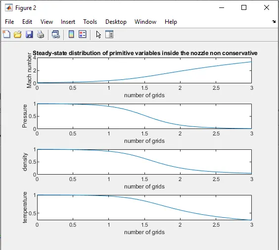
Steady-state distribution of primitive variables inside the nozzle for non-conservative form.

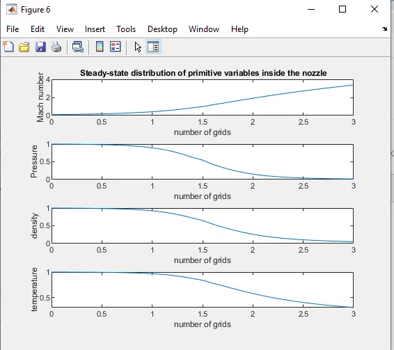
Steady state distribution of the primitive variables inside the nozzle that is density, presssure, temperature, and Mach numberfor conservative form.

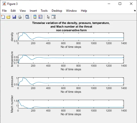
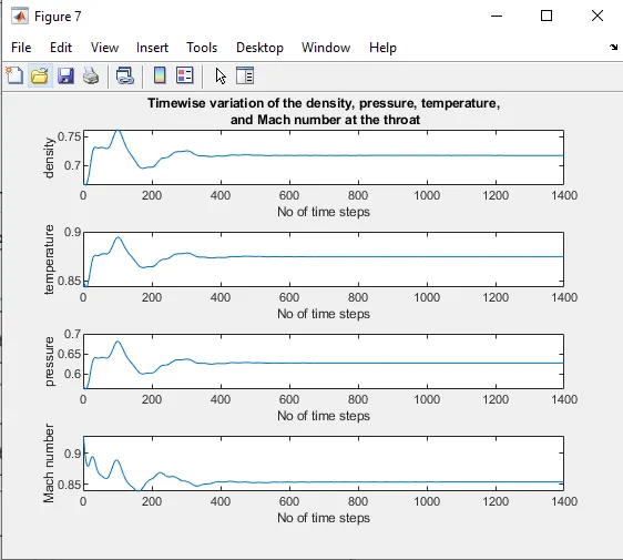
Timewise Variation of primitive variables with the time that is density, pressure, temperature, and Mach number at the throat for non-conservative form.

Timewise Variation of primitive variables with the time that is density, pressure, temperature, and Mach number at the throat for conservative form.

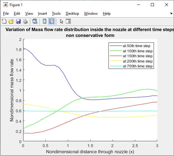
Variation of the mass flow rate at different time steps can be observed for the non-conservative form in the below graph. For the 1400 number of time steps at the time steps 50, 100, 150, 200, and 700 the plots are shown in the figure.

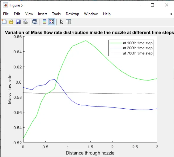
Variation of the mass flow rate at different time-steps for conservation form. For the number of time step 1400 the plots are made for 100, 200, 700 time step.

Comparison of Normalized mass flow rate distributions of both conservative and non-conservative forms.

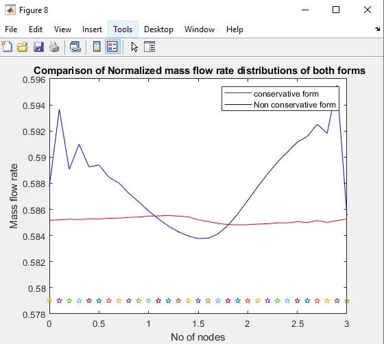
In the above plot,we compare the steady state variations of mass flow obtained with the non-conservative and conservative forms of the governing equations.Here we see that the steady state mass flow distribution predicted by the conservative form of the equations is much more satisfactory than that obtained from the non-conservative form ,on two accounts.

1.The conservative form gives a distribution i.e much closer to being a constant.In contrast,the non-conservative results have a sizeable variation with some oscillations at both the inflow and outflow boundary of course on a practical basis,these variations are not apparent and the mass flow essentially appears to be constant.

2.The steady state mass flow results obtained with the conservative form are,on the whole,much closer to the exact analytical solution.(rho'A'V'=0.579).

comparision of Conservation and non-conservation form for grid independence test.

No.of grids	Method	ρ	t	P	M
31	Conservation	0.6340	0.8330	0.534	0.999
31	non-conservation	0.6505	0.8365	0.546	0.9816
61	Conservation	0.6383	0.8330	0.533	0.9993
61	non-conservation	0.6340	0.8975	0.5326	0.999

The above discussion does not necessarily establish a definite superiority of the conservative form results over the non-conservative form result,let us look at the primitive variables in particular density,temperature ,pressure and mach number at nozzle throat as tabulated in the above table.By doubling the number of grid points the steady stae numerical results are slighlty closer to the exact,analytical values.for all the particular purposes we have grid independence with 31 grid points suppose to produce the steady state results.

CONCLUSION.

From this challenge we can observe that both the conservative and the non-conservative forms are analytically same but when we see the results in the indepenence grid test the conservative form results are not varying much means we can see the very little amount of changes in the values for the primitive variables as well as in the non-convservation form also the same thing we can observe but as we compare to conservation form the changes are slight more in the non-conservation form but not so much for both the form so we can observe that the primitive variables that are pressure, density, temperature, and Mach number are not varying so much when we double the number of grids for both 31 and 61 number of grids the values are almost the same.