Week 7 - Simulation of a 1D Super-sonic nozzle flow simulation using Macormack Method

Week 7 - Simulation of a 1D Super-sonic nozzle flow simulation using Macormack Method

GIVEN PROBLEM:

In this challenge you are going to simulate the isentropic flow through a quasi 1D subsonic-supersonic nozzle. You will derive both the conservation and non-conservation forms of the governing equations and sovle them using the MacCormack's technique. You need to determine the steady-state temperature distribution for the flow-field variables and investigate the difference between the two forms of governing equations by comparing their solutions.

You need to show the following plots inside your report
1. Steady-state distribution of primitive variables inside the nozzle
2. Time-wise variation of the primitive variables
3. Variation of Mass flow rate distribution inside the nozzle at different time steps during the time-marching process
4. Comparison of Normalized mass flow rate distributions of both forms

Expected Results:

• Perform a grid independence test on the solution and expain all your findings.
• The code must be modular. You need to write separate functions to solve both forms.
• Discuss all the plots you are providing with observed inferences.

OBJECTIVE:

The work is focused on writting a matlab/octave code to simulate the isentropic flow through a quasi one dimensional supersonic nozzle for boh conservative and non conservative forms of governing equations and solving them using MacCormacks technique and compare their solutions by performaing a grid dependancy test.Through this project report we will compre some important theory concept such as : What is nozzle? What is supersonic flow and how do we define it in a C-D nozzle? What is MaCcromac method and which governing equation weare using?The programme will be divided into three parts , It will have a main programme script followed by two separate user defined function(UDF) one for conservative form and other for non conservative form of governing equation which will be called in the main MATLAB/OCTAVE code.

THEORY:

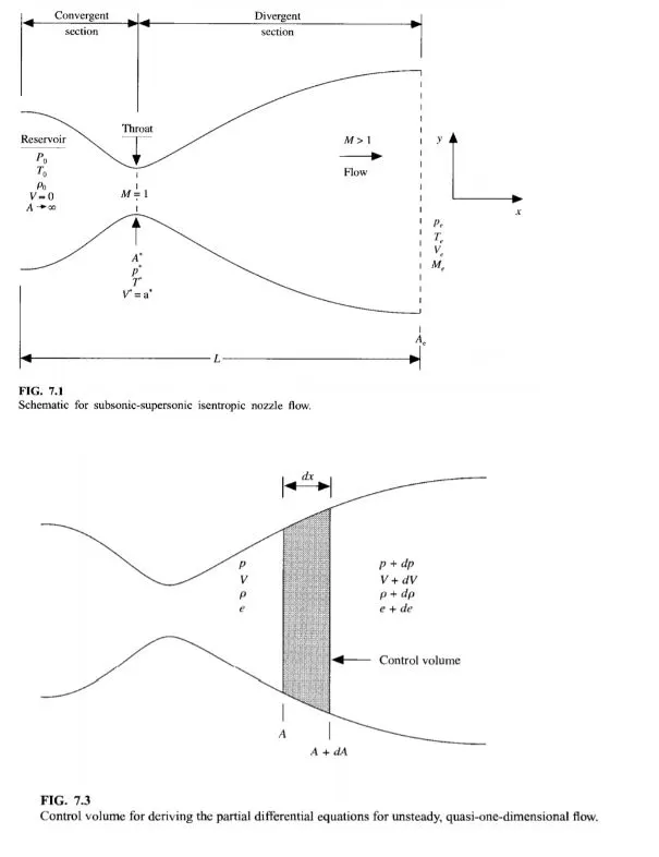
Ramjets,scramjets and rockets all use nozzles to accelerate hot exaust to produce forward thrust as described by newtons third law of motion i.e. for every action there is equal and opposit rection . The ammount of thrust produced by the engine

depends on the mass flow rate(m'=(dm/dt) where m'=mass flow rate, dm=change in mass, dt=change in time) through the engine .The value of these flow variables are determined by the nozzle design . A nozzle is a relatively simple device , just aspecially shaped tube through hot gases flow.Ramjets and rockets typically use a fixed convergent section followed by afixed divergent section for the design of the nozzle. This nozzle configeration is called a convergent-divergent or cd ,nozzle.In Cd nozzle the hot exhaust leaves the combuction chamber and converges down to minimum area , or throat of the nozzle.The throat size is chosen to choke the flow and set the mass flow rate through the system.The flow in the throat is sonic i.e. Mach NUMBER(M) is equal to one in the throat. Downastream of the throat the geomatry diverges and the lfow is isentropically expanded to supersonic mach number that depends on the area ratio at the exit of the throat.The expansion of the supersonic flow causes the static pressure and temperature to decrease from the throat to the exit, so the ammount of expansion determines the exit pressure and temperature . The exit temperature determines the exit speed of the sound ,which determines the exit veloity.The exit velocity, pressure and mass flow through the nozzle determine sthe ammount of thrust produced by the nozzle.

.conservation of mass equation: m' =rho*A*V where m'=mass flow rate, rho=Gas density, A=cross section of flow area

V=gas velocity

.conservation of momentum equation : rho*V*dV=-dp

.Isentropic flow relation :(dp/p)=(gamma)*(drho/rho) where gamma is defined as the ratio of specfic heats(Cp/Cv) for air , where gamma=1.4.

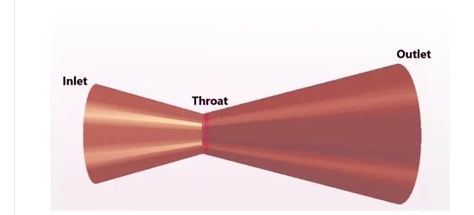
Quasi and dimensional implies that we still have variations of flow quantities in one direction only but we allow the cross section area of yhe steam tubes to vary along the same direction as well . This means that we are able to analyze axisymmetric channels with varying cross section areas such as convergent-divergent nozzle.

A gas is forced through through the tube and gas molecules get deflected by the walls of the tube . If speed of the gas is much less than the speed of sound , the density of the gas remains constant and the velocity of flow increases . however ,as the speed of flow approaches the speed of sound we msut consider compressibility effects on the gas.The density of gas varies from one location to another.considering the flow throagh the ube as shown in the figure,if the flow vary gradually compressed(area decreases),the flow conditions return to the original values. We say that such a process is reversible.From the consideration of the second law of thermodynamics , a reversible flow maintains a constant value of entropy.Engineers called the type of flow as isentropic flow. Isentropic flow occures when the change in flow variable is small and gradual,such as ideal flow through the nozzle shown above.The ratio of speed of aircaft and speed of sound in the gas determine sthe magnitude of many compressibility effects.Because of the importance of the speed ratio the aerodynamicities have designed it with a special parameters called MACH number . The mach number M allows us to define flight reims in which compressibility effects vary.

M=(object speed /speed of sound)

1. Subsonic conditions occur for mach number condition less than one ,M<1. For the lowest subsonic conditions compressibility can be ignored.

2.As the speed of object approaches the speed of sound , the flight mach number is near equal to one,M=1,and the flow said to be transonic.At some places of the object the local speed exceeds the speed of sound. The compressibility effect is most important in transonic flow and lead to early belief in a sound barrier. The flight faster than was thought to be impossibile. In fact the sound barrier was only the increase in the drag near sonic onditions because of compressibility effects. Because of highn drag associtedc with compressibility effects, aircraft can not cruise near mach 1.

3.supersonic conditions occure because of mach number graeter than one,1<M<3. compressibility effect is important for supersonic aircraft and shock waves are generated because of the surface of the object.For very high supersonic speed , 3<M<5 ,aerodynamic heating is very important for aircraft design .

4. For speed greter than 5 times the speed of sound ,M>5, he flow is said to be hypersonic .At this speed some of the energy of the object now gose into exiciting the chemical bonds which hold together the nitrogen and oxygen molecules of air. At hypersonic speed the chemistry of air must be considered when determining the forces on the object.The space shuttels re enter the atmosphere at high hypersonic speed,M~25. In this condition the heated air becomes an ionized plazma of gas and the spacecraft must be insulated from high temperatures.

continuity equation , Navier-stokes equation and enrgy equation are the key governing equation that indicates the hpysics of fluid mechanics and thermal sciences, which are instrumental in the research of computational fluid dynamics(CFD).The governing equations stem from fundamental principle of the newtons law and Renolds transport theorem which can be expressed into a general form of integral equation. howver such ageneral form is not conventional for presise analysis down to the scale of fluid element percels.The eulerian approach therefore takes the stage and it further developed into the differential form of equations that involves tensor and indical notation for spectial description and flow fields .

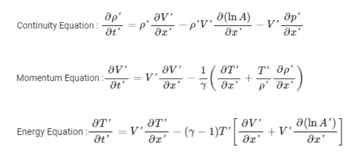
NON-CONSERVATIVE FORM OF GOVERNING EQATIONS:

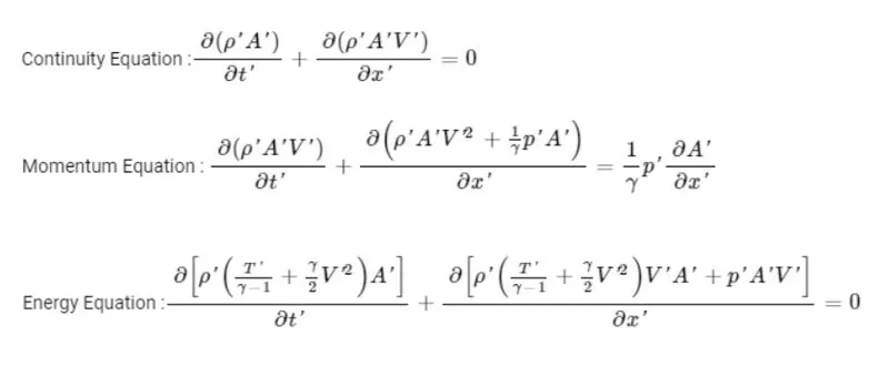
CONSERVATIVE FORM OF GOVERNING EQUATIONS:

In CFD the MacCromac method is widely uesd discretization scheme for the numerical solution of hyperbolic pertial differential equation . MacCromac method[1, 2] is a predictor corrector finite difference scheme that has been used for compressible flow and other application for over twenty years. There exist both implicit and xeplicit versions of the algorithm but the xeplicit predates the implicit by more than a decade nad it is considered one of the milestone of the computational fluid dynamics.Both versions facilitates the solutions of hyperbolic an parabolic by merching forward in time.The applications of the MaCcromac method is done im two steps : A predictor step which is followed by a corrector step. To illustrate the algorithm consider the following hyoerbolic equtaion :

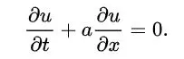
PREDICTOR STEP: In predictor step a provisonal value of 'u' at time 'n+1' denoted by

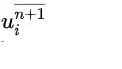
is estimated as follows

The above equation is obtained by replacing the special and temporal derivatives in the previous first order hyperbolic equation using forward difference.

CORRECTOR STEP: In the corrector step the predicted value{discplay u_{i}^{overline{n+1}}}

is corrected according to the equation

Note that the corrector step uses the bacward finite difference approximation for spatial derivative. The time term used in the correcrtor step is Δt/2 incontrast to the Δt used in predictor step . Replacing the

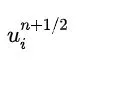
term by the temporal average

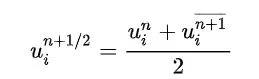
to obtain corrector step as

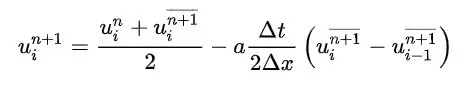
Apply predictor step to the Non-conservative form of governing equations

Find time derivative value at all the points

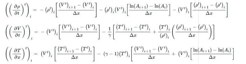
Apply corrector step to the non conservative form of governing equation

Find time derivative values at time (t+dt) with predictor values.

similarly we can compute the predictor step and corrector step of the conservative form of the governing equations as well.

CODE:

FUNCTION CODE(NON-CONSERVATIVE):

function [mass_flow_rate_nc,pressure_nc,mach_number_nc,rho_nc,v_nc,T_nc,rho_throat_nc,v_throat_nc,T_throat_nc,mass_flow_rate_throat_nc,pressure_throat_nc,mach_number_throat_nc]=non_consarvative_form(x,dx,n,gamma,nt,c)
% initial boundary condition
rho_nc=1-0.3146*x;
T_nc=1-0.2341*x;
v_nc=(0.1+1.09*x).*T_nc.^0.5;
% Area and throat profiles
a=1+2.2*(x-1.5).^2;
throat=find(a==1)

% outer time loop
for k=1:nt
    % Time step control
    dt=min(c.*dx./(sqrt(T_nc)+v_nc));

    % saving a copy of old values
    rho_old=rho_nc;
    T_old=T_nc;
    v_old=v_nc;

    % predictor method
    for j=2:n-1

        %simplyfing the equations special terms
        dv_dx=(v_nc(j+1)-v_nc(j))/dx;
        drho_dx=(rho_nc(j+1)-rho_nc(j))/dx;
        dT_dx=(T_nc(j+1)-T_nc(j))/dx;
        dlog_a_dx=(log(a(j+1))-log(a(j)))/dx;
        % continuity equation
        drho_dt_p(j)=-rho_nc(j)*dv_dx-rho_nc(j)*v_nc(j)*dlog_a_dx-v_nc(j)*drho_dx;

        % Momentum equation
        dv_dt_p(j)=-v_nc(j)*dv_dx-(1/gamma)*(dT_dx+(T_nc(j)*drho_dx/rho_nc(j)));

        % Energy equation
        dT_dt_p(j)=-v_nc(j)*dT_dx-(gamma-1)*T_nc(j)*(dv_dx+v_nc(j)*dlog_a_dx);

        %solution update
        rho_nc(j)=rho_nc(j)+drho_dt_p(j)*dt;
        v_nc(j)=v_nc(j)+dv_dt_p(j)*dt;
        T_nc(j)=T_nc(j)+dT_dt_p(j)*dt;
    end

    % Corrector method
    for j=2:n-1
          %simplyfing the equations special terms
          dv_dx=(v_nc(j)-v_nc(j-1))/dx;
          drho_dx=(rho_nc(j)-rho_nc(j-1))/dx;
          dT_dx=(T_nc(j)-T_nc(j-1))/dx;
          dlog_a_dx=(log(a(j))-log(a(j-1)))/dx;

           % continuity equation
        drho_dt_c(j)=-rho_nc(j)*dv_dx-rho_nc(j)*v_nc(j)*dlog_a_dx-v_nc(j)*drho_dx;

        % Momentum equation
        dv_dt_c(j)=-v_nc(j)*dv_dx-(1/gamma)*(dT_dx+(T_nc(j)*drho_dx/rho_nc(j)));

        % Energy equation
        dT_dt_c(j)=-v_nc(j)*dT_dx-(gamma-1)*T_nc(j)*(dv_dx+v_nc(j)*dlog_a_dx);
    end

    % compute average time derivative
    dro_dt=0.5*(drho_dt_p+drho_dt_c);
    dv_dt=0.5*(dv_dt_p+dv_dt_c);
    dT_dt=0.5*(dT_dt_p+dT_dt_c);

    % Final solution update
    for i=2:n-1
        rho_nc(i)=rho_old(i)+dro_dt(i)*dt;
        v_nc(i)=v_old(i)+dv_dt(i)*dt;
        T_nc(i)=T_old(i)+dT_dt(i)*dt;
    end

    % Applying boundary conditions
    % At inlet
    rho_nc(1)=1;
    v_nc(1)=2*v_nc(2)-v_nc(3);
    T_nc(1)=1;

    % At outlet
    rho_nc(n)=2*rho_nc(n-1)-rho_nc(n-2);
    v_nc(n)=2*v_nc(n-1)-v_nc(n-2);
    T_nc(n)=2*T_nc(n-1)-T_nc(n-2);

    % Defining mass flow rate, presure and Mach number
    mass_flow_rate_nc=rho_nc.*a.*v_nc;
    pressure_nc=rho_nc.*T_nc;
    mach_number_nc=(v_nc./sqrt(T_nc));

    % calculating variables at throat section
    rho_throat_nc(k)=rho_nc(throat);
    T_throat_nc(k)=T_nc(throat);
    v_throat_nc(k)=v_nc(throat);
    mass_flow_rate_throat_nc(k)=mass_flow_rate_nc(throat);
    pressure_throat_nc(k)=pressure_nc(throat);
    mach_number_throat_nc(k)=mach_number_nc(throat);

    % ploting
    % comparison of non-dimensional mass flow rate at different timestep
    figure(1);
    if k==50
        plot(x,mass_flow_rate_nc,'m','linewidth',1.25);
        hold on
    elseif k==100
         plot(x,mass_flow_rate_nc,'c','linewidth',1.25);
    elseif k==200
         plot(x,mass_flow_rate_nc,'g','linewidth',1.25);
    elseif k==400
         plot(x,mass_flow_rate_nc,'y','linewidth',1.25);
    elseif k==800
         plot(x,mass_flow_rate_nc,'k','linewidth',1.25);
         hold on
    end
       % Labeling
    title('Mass flow rate at different timesteps-non-Conservative form')
    xlabel('Distance')
    ylabel('Mass Flow Rate')
    
    axis([0 3 0.4 1])
    grid on
end
legend({'50^t^h timestep','100^t^h timestep','200^t^h timestep','400^t^h timestep','800^t^h timestep'});

end







     

EXPLANATION:

• The purpose of the function is to calculate the values of mass flow rate ,pressure,velocity,density,Temperature and Density at the throat,Velocity at the throat,pressure at the throat,Temperature at the throat,mass flow rate at the throat,mach number at the throat by the known equations at all the grid points(n=31). To determine the initial profile of Density and Temperarure for loop is used inputing the know conditions using the else-if command.
• For the initial boundary conditions are established for density,Temperature and velocity profiles for calculating area and throat.
• Now our time loop is computed for the loop to calculate all the grid points for various formulas inside the loop.
• MaCcromac technique is used to solve the numerical solution of governing equations such as Continuity, Momentum and energy equation.
• The technique implies two methods for solving namely predictor method followed by corrector method.
• The predictor and corrector methods are assigned within the for loop individual for calculating values.
• The calculated values are averaged in the next step and updating solution with old values.
• Boundary conditions are applied within the for loop and subsquently used for calculating the Mass flow rate , Mach number and pressure and calculating values at the throat section.
• Finally ploting is done for Distance(x) and mass flow rate for different timesteps.
• The programme is ended.

FUNCTION CODE(CONSERVATIVE):

function [mass_flow_rate_c,pressure_c,mach_number_c,rho_c,v_c,T_c,rho_throat_c,v_throat_c,T_throat_c,mass_flow_rate_throat_c,pressure_throat_c,mach_number_throat_c]=consarvative_form(x,dx,n,gamma,nt,c)
% Determining initial profile of density and temperature
for i=1:n

    if(x(i)>=0 && x(i)<=0.5)
        rho_c(i)=1;
        T_c(i)=1;
    elseif (x(i)>=0.5 && x(i)<=1.5)
        rho_c(i)=1-0.366*(x(i)-0.5);
        T_c(i)=1-0.167*(x(i)-0.5);
    elseif (x(i)>=1.5 && x(i)<=3)
        rho_c(i)=0.634-0.3879*(x(i)-1.5);
        T_c(i)=0.833-0.3507*(x(i)-1.5);
    end
end
% area & throat profiles
a=1+2.2*(x-1.5).^2;
throat=find(a==1);

% Initial profile for velocity and pressure
v_c=0.59./(rho_c.*a);
pressure_c=rho_c.*T_c;
% calculate the initial solution vector(U)
u1=rho_c.*a;
u2=rho_c.*a.*v_c;
u3=rho_c.*a.*(T_c./(gamma-1))+((gamma/2).*v_c.^2);

%outer time loop
for k=1:nt

    % Time step control
    dt=min(c.*dx./(sqrt(T_c)+v_c));

    % saving the copy of old values
    u1_old=u1;
    u2_old=u2;
    u3_old=u3;

    % calculating the flux vectoe
    F1=u2;
    F2=((u2.^2)./u1)+((gamma-1)/gamma)*(u3-(gamma/2)*((u2.^2)./u1));
    F3=((gamma*u2.*u3)./u1)-(gamma*(gamma-1)*((u2.^3)./(2*u1.^2)));

    %predictor method
    for j=2:n-1
        
        %calculatign the source term
        j2(j)=(1/gamma)*rho_c(j)*T_c(j)*((a(j+1)-a(j))/dx);

        %continuity equation
        du1_dt_p(j)=-((F1(j+1)-F1(j))/dx);
        % Momentum equation
        du2_dt_p(j)=-((F2(j+1)-F2(j))/dx)+j2(j);

        % Energy equation
        du3_dt_p(j)=-((F3(j+1)-F3(j))/dx);

        %updating new values
        u1(j)=u1(j)+du1_dt_p(j)*dt;
        u2(j)=u2(j)+du2_dt_p(j)*dt;
        u3(j)=u3(j)+du3_dt_p(j)*dt;

    end

    % updating flux vector
    F1=u2;
    F2=((u2.^2./u1)+((gamma-1)/gamma)*(u3-((gamma*0.5*(u2.^2))./u1)));
    F3=((gamma*u2.*u3)./u1)-((gamma*0.5*(gamma-1)*(u2.^3))./(u1.^2));

    % corrector method
    for j=2:n-1

        %updating source term
        j2(j)=(1/gamma)*rho_c(j)*T_c(j)*((a(j)-a(j-1))/dx);

        % simplying the Equations special terms
        du1_dt_c(j)=-((F1(j)-F1(j-1))/dx);
        du2_dt_c(j)=-((F2(j)-F2(j-1))/dx)+j2(j);
        du3_dt_c(j)=-((F3(j)-F3(j-1))/dx);
    end

    % compute average time derivative
    du1_dt=0.5*(du1_dt_p+du1_dt_c);
    du2_dt=0.5*(du2_dt_p+du2_dt_c);
    du3_dt=0.5*(du3_dt_p+du3_dt_c);

    % final solution update
    for i=2:n-1
        u1(i)=u1_old(i)+du1_dt(i)*dt;
        u2(i)=u2_old(i)+du2_dt(i)*dt;
        u3(i)=u3_old(i)+du3_dt(i)*dt;
    end

    % Applying boubdary condition
    % At inlet
    u1(1)=rho_c(1)*a(1);
    u2(1)=2*u2(2)-u2(3);

    v_c(1)=u2(1)./u1(1);
    u3(1)=u1(1)*((T_c(1)/(gamma-1))+((gamma/2)*(v_c(1)).^2));

    % At outlet
    u1(n)=2*u1(n-1)-u1(n-2);
    u2(n)=2*u2(n-1)-u2(n-2);
    u3(n)=2*u3(n-1)-u3(n-2);

    % Final primitive value update
    rho_c=u1./a;
    v_c=u2./u1;
    T_c=(gamma-1)*((u3./u1-(gamma/2)*(v_c).^2));
    % Defining mass flow rate , pressure and mach number
    mass_flow_rate_c=rho_c.*a.*v_c;
    pressure_c=rho_c.*T_c;
    mach_number_c=(v_c./sqrt(T_c));
    
    % calculating variables at the throat section
    rho_throat_c(k)=rho_c(throat);
    T_throat_c(k)=T_c(throat);
    v_throat_c(k)=v_c(throat);
    mass_flow_rate_throat_c(k)=mass_flow_rate_c(throat);
    pressure_throat_c(k)=pressure_c(throat);
    mach_number_throat_c(k)=mach_number_c(throat);

    %ploting
    % comparison of non dimensional mass flow rates at different timesteps
    figure(4)
    if k==50
        plot(x,mass_flow_rate_c,'m','LineWidth',1.25)
        hold on
    elseif k==100
        plot(x,mass_flow_rate_c,'c','LineWidth',1.25)
    elseif k==200
        plot(x,mass_flow_rate_c,'g','LineWidth',1.25)
    elseif k==400
        plot(x,mass_flow_rate_c,'y','LineWidth',1.25)
    elseif k==800
        plot(x,mass_flow_rate_c,'k','LineWidth',1.25)
        hold on
    end

    % Labeling
    title('Mass flow rate at different timesteps-Conservative form')
    xlabel('Distance')
    ylabel('Mass Flow Rate')
  
    axis([0 3 0.4 1])
    grid on
end
  legend({'50^t^h timestep','100^t^h timestep','200^t^h timestep','400^t^h timestep','800^t^h timestep'});
end

EXPLANATION:

• The purpose of the function is to calulate the values of Mass flow rate,Pressure,Mach number ,Density ,velocity,Temperature and Density at the throat,velocity at the throat, pressure at the throat,Mass flow rate at the throat, Mach number at the throat by the known equations for the all grid points(n=31).To determine the initial profiles of Density and Temperature for loop is used inputing the known conditions within an else-if command.
• Initial values of area ,throat, velocity and pressure are calulated using formulas.
• In order to simplify and avoid errors the equation is divided into solution vector (U),Flux vector(F) and source term(j).
• New outer time loop is computed for the loop to calculate all the grid points for various formulas inside the loop.
• MaCcromac technique is used to solve numerical solution of governing equations such as continuity ,momentum and energy equation.
• The techinque implies two methods for solving namely predicto method followed by corrector method.
• predictor and corrector methods are assigned within the for loop individually for calculating the values.
• The calculated values are averaged in the next step and updating the solutions with old values .
• Boundary conditions are applied within the for loop and subsquently used for calculating the Mass flow rate, pressure and Mach number and also calculating the values at the throat section.
• Finally ploting is done for Distance(x) and Mass flow rate at different time step.
• The programme is ended.

MAIN CODE:

clear all
close all
clc
% Input parameters
n=31;
gamma=1.4;
x=linspace(0,3,n);
dx=x(2)-x(1);

% no of timestep
nt=1400;

%courant number
c=0.5;

% Funxtion for non conservative form
tic;
[mass_flow_rate_nc,pressure_nc,mach_number_nc,rho_nc,v_nc,T_nc,rho_throat_nc,v_throat_nc,T_throat_nc,mass_flow_rate_throat_nc,pressure_throat_nc,mach_number_throat_nc]=non_consarvative_form(x,dx,n,gamma,nt,c)
Time_elapsed_nc=toc;
fprintf('Time elapsed non conservativ form: %0.4f',Time_elapsed_nc);
hold on
% ploting
% Timestep variation of properties at throat section in non consercvatie
% form
figure(2)
% Density
subplot(4,1,1)
plot(linspace(1,nt,nt),rho_throat_nc,"Color",'m','LineWidth',2)
ylabel('Density')
legend({'Density at throat'})
axis([0 1400 0 1.3])
grid minor;
title('Timestep variation at throat area Non-conservative Form')

% Temperature
subplot(4,1,2)
plot(linspace(1,nt,nt),T_throat_nc,"Color",'c','LineWidth',2)
ylabel('Temperature')
legend({'Temperature at throat'})
axis([0 1400 0.6 1])
grid minor;

% pressure
subplot(4,1,3)
plot(linspace(1,nt,nt),pressure_throat_nc,"Color",'g','LineWidth',2)
ylabel('Pressure')
legend({'Pressure at throat'})
axis([0 1400 0.4 1.1])
grid minor;

% Mach number
subplot(4,1,4)
plot(linspace(1,nt,nt),mach_number_throat_nc,"Color",'y','LineWidth',2)
ylabel('Mach number')
legend({'Mach number at throat'})
axis([0 1400 0.6 1.4])
grid minor;

% Steady state simulation for primitive values of non conservative form
figure(3)
% Density
subplot(4,1,1)
plot(x,rho_nc,"Color",'c','LineWidth',2)
ylabel('Density')
legend({'Density'});
axis([0 3 0 1])
grid minor;
title('variation of flow rate distribution-non-conservative')

% Temperature
subplot(4,1,2)
plot(x,T_nc,"Color",'m','LineWidth',2)
ylabel('Temperature')
legend({'Temperature'});
axis([0 3 0 1])
grid minor;

% pressure
subplot(4,1,3)
plot(x,pressure_nc,"Color",'g','LineWidth',2)
ylabel('Pressure')
legend({'pressure'});
axis([0 3 0 1])
grid minor;

% Mach number
subplot(4,1,4)
plot(x,mach_number_nc,"Color",'y','LineWidth',2)
ylabel('Mach number')
legend({'Mach number'});
axis([0 3 0 1])
grid minor;

% Function for conservative form
tic;
[mass_flow_rate_c,pressure_c,mach_number_c,rho_c,v_c,T_c,rho_throat_c,v_throat_c,T_throat_c,mass_flow_rate_throat_c,pressure_throat_c,mach_number_throat_c]=consarvative_form(x,dx,n,gamma,nt,c)
Time_elapsed_c=toc;
fprintf('Time elapsed for conservative form: %0.4f',Time_elapsed_c);

% ploting
% Time variation for properties at throat area of conservative form
figure(5)

% Density
subplot(4,1,1)
plot(rho_throat_c,'color','m','LineWidth',2)
ylabel('Density')
legend({'Density at throat'});
axis([0 1400 0 1]);
grid minor;
title('Timestep variation at throat area-conservative form')

% Temperature
subplot(4,1,2)
plot(T_throat_c,'color','c','LineWidth',2)
ylabel('Temperature')
legend({'Temperature at throat'});
axis([0 1400 0.6 1.2]);
grid minor;

% pressure
subplot(4,1,3)
plot(pressure_throat_c,'color','g','LineWidth',2)
ylabel('pressure')
legend({'pressure at throat'});
axis([0 1400 0.2 0.8]);
grid minor;

% Mach number
subplot(4,1,4)
plot(mach_number_throat_c,'color','y','LineWidth',2)
ylabel('pressure')
legend({'pressure at throat'});
axis([0 1400 0.6 1.4]);
grid minor;

% Steady state simulation for primitive value of conservative form
figure(6)
% Density
subplot(4,1,1)
plot(x,(rho_c),"Color",'c','LineWidth',2)
ylabel('Density')
legend({'Density'});
axis([0 3 0 1])
grid minor;
title('variation of flow rate distribution-conservative')

% Temperature
subplot(4,1,2)
plot(x,(T_c),"Color",'m','LineWidth',2)
ylabel('Temperature')
legend({'Temperature'});
axis([0 3 0 1])
grid minor;

% pressure
subplot(4,1,3)
plot(x,(pressure_c),"Color",'g','LineWidth',2)
ylabel('Pressure')
legend({'pressure'});
axis([0 3 0 1])
grid minor;

% Mach number
subplot(4,1,4)
plot(x,(mach_number_c),"Color",'y','LineWidth',2)
ylabel('Mach number')
legend({'Mach number'});
axis([0 3 0 4])
grid minor;

% comparison plot for normalized mass flow rate of both forms
figure(7)
hold on
plot(x,mass_flow_rate_nc,'r','LineWidth',2)
hold on
plot(x,mass_flow_rate_c,'b','LineWidth',2)
hold on;
grid on

legend('non-conservative','conservative') % compare
xlabel('length of the domain')
ylabel('mass flow rate')
title('comparison of normalized mass flow rate of both forms')

EXPLANATION:

• Code start with clear, close,clc which enables fresh start of a new programme without the manipulation of the previous value.
• Input parameters are assigned for variables x,dx,n,gamma,nt,c.
• Non conservative and conservative forms are created with separate functions with necessary inputs
• The "tic toc" command is used for calculating the time elapsed between the functions.
• ploting is done for the following solutions:1. Timestep variation at throat area at both the form,2. Variation of flow rate distribution at both the form,3.comparison of normalized mass flow rate at both the form.
• Eah plot is computed as subplot of four primitive variables such as Density, Pressure,Temperature and Mach number at the throat of the nozzle as well as the convergent divergent section.

RESULTS:

1. Plots for time variation at the throat for both conservative and non conservative forms of governing equation

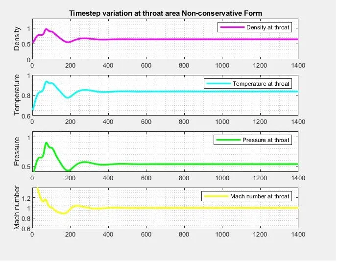
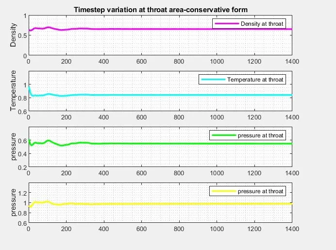
From the above plots we can see that the solution has reached a stable solution for 200 iteration for conservation form and 400 iteration for non conservative form for the same grid points.For non conservative form of governing equation we can see few derivation at the initial phase which lead to a longer time to converge .Therefore we can conclude that conservative form of governing equation give us quicker solution than that of the non conservative form.

2.Plots for variation of flow rate distribution for both conservative and non conservative forms of governing equation:

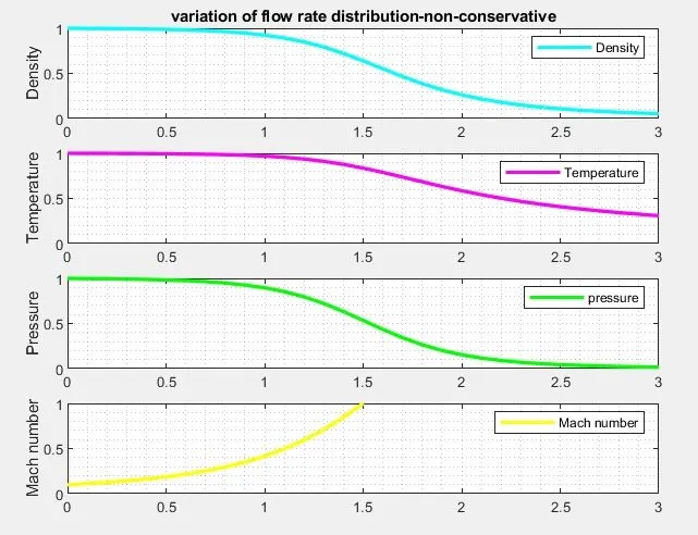
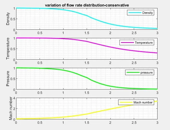
Form the above plots we can obaserve that for both conservative and non conservative form of governing equations flow rate distribution of Density, Temperaur,Pressure and Mach number is quite similer.

3.Plots for mass flow rate at different timestep for both conservative and non con servative form of governing equation:

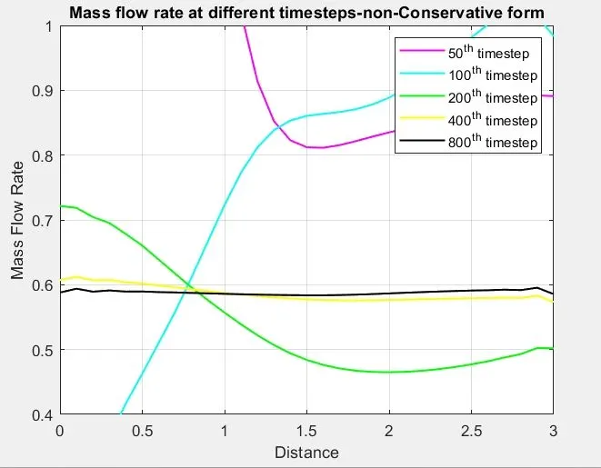
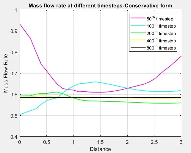
From the above plots we can observe that the mass flow rate at the outlet for different timestep. Initially the plots oscillate and become unstable till 200 th timestep then became stable and reachde convergence for both conservative and non conservative form.

4.Plot for comparing mass flow rate for both conservative and non conservative form of governing equation:

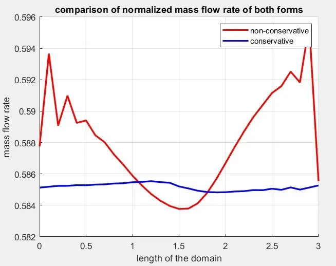
From the above plot we can conclude that the conservative form of governing equation attains stability in lesser number of iteration than non conservative form of governing equation.

ERROR OCCURED:

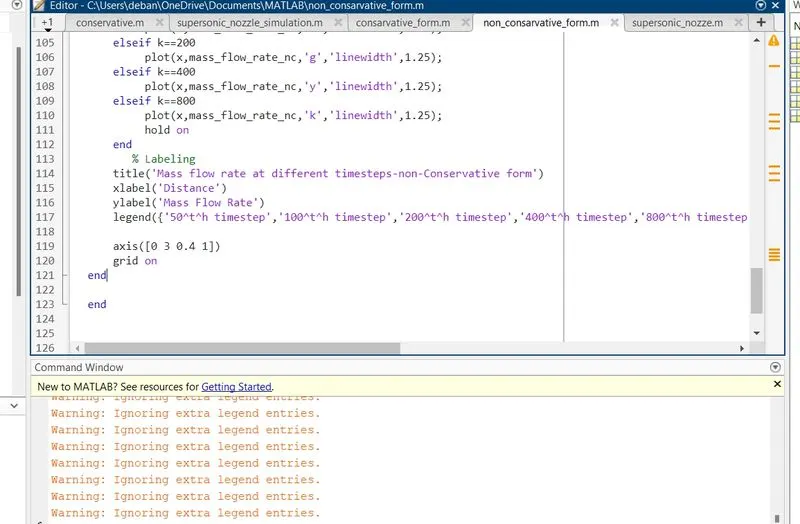
error occured :warning:ignoring extra legend entries as the legend is taken within the time loop so when it start calculating iteration say at 200 then legend entries are more than that so to solve the problem take legend out of loop for both conservative and non conservative function.

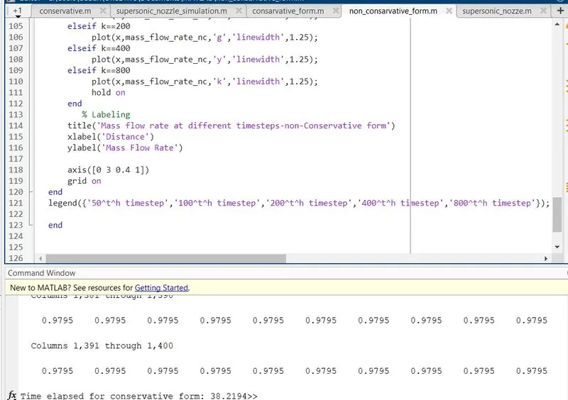
Then no error occured

Grid Dependency is an important factor where we try to improve the solution by improving the mesh quality (adding more cells) ,so for our case we increased the number of grid points from 31 to 61 and populated them in a sheet and run the code again .upon running the simulation it is observed that the values are similar or the primitive variables for both the forms even when the grid points (n)are changed from 31 to 61 showcasing that it dose not get affected by increase of the grid points .Hence we can conclude that the solution is grid independent.