Week 7 - Simulation of a 1D Super-sonic nozzle flow simulation using Macormack Method
AIM:- Simulating quasi 1-D flow through a converging diverging nozzle using macCormack method.
THEORY
A nozzle is a type of device designed to control the direction or characterstics of fluid flow at the exit of pipe . A nozzle is often a pipe or tube of varying cross sectional area, thus can be used to direct or modify flow of fluid.
A convergent - divergent nozzle is a device used to accelerate a hot , pressurised gas passing through it to be higher supersonic speed in the axail direction by converting heat energy of the flow to kinetic energy.Hence such nozzles are used in steam turbines, supersonic jets engines.
In this project the problem is taken from the Jd Anderson book on CFD
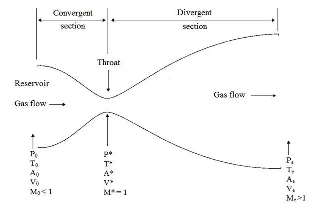
The symmetrical area function for the CD nozzle is given as,
`(A/A^**)^2 = 1 + 2.2(x - 1.5)^2`
Where `A^**` is the area at the throttle and x is distance along the length of nozzle.
The non-dimensional form of the variables required for this problem are:-
`x' = x/L; V' = V/a_0; t' = t/(L/a_0); rho' = (rho)/(rho_0); T' = T/T_0; p' = p/p_0; A' = A/(A^**)`
GOVERNING EQUATIONS
1. NON-CONSERVATION FORM
The non-conservation form of governing equation which represents continuity momentum & Energy in terms of non dimensional variables
Continuity: `(delrho')/(delt') = - rho'(delV')/(delx') - rho'V'(del(lnA'))/(delx') - V'(delrho')/(delx')`
Momentum: `(delV')/(delt') = - V'(delV')/(delx') - 1/(gamma)[(delT')/(delx') + (T')/(rho') (delrho')/(delx')]`
Energy: `(delT')/(delt') = - V'(delT')/(delx') - (gamma-1)T' [(delV')/(delx') + V' (del(lnA'))/(delx')]`
The initial conditions are
`rho'(t=0) = 1 - 0.3146x'`
`T'(t=0) = 1 - 0.2314x'`
`V'(t=0) = (0.1 + 1.09x')sqrt(T'(t=0))`
2. CONSERVATION FORM
The conservational form equation represents continuity,momentum & energy in non-dimensional form is given as
Continuity: `(del(rho'A'))/(delt') + (del(rho'A'V'))/(delx') = 0`
Momentum: `(del(rho'A'V'))/(delt') + (del(rho'A'V'^2 + (1/(gamma))p'A'))/(delx') = 1/(gamma) p' (delA')/(delx')`
Energy: `(del[rho'((T')/(gamma-1) + (gamma)/2 V'^2)A'])/(delt') + (del[rho'((T')/(gamma-1) + (gamma)/2 V'^2)V'A' + p'A'V'])/(delx') = 0`
In order to simplify these equations we substitute following term includes solution vectors `U_i` , the flux vector `F_i` and source term `J_2`.
`U_1 = rho'A'`
`U_2 = rho'A'V'`
`U_3 = rho'[(T')/(gamma-1) + (gamma)/2 V'^2]A'`
`F_1 = rho'A'V' = U_2`
`F_2 = rho'A'V'^2 + 1/(gamma) p'A' = (U_2^2)/(U_1) + (gamma-1)/(gamma) [U_3 - (gamma)/2 (U_2^2)/(U_1)]`
`F_3 = rho'((T')/(gamma-1) + (gamma)/2 V'^2)V'A' + p'A'V' = gamma (U_2U_3)/U_1 - (gamma(gamma-1))/2 (U_2^3)/(U_1^2)`
`J_2 = 1/(gamma) p' (delA')/(delx')`
After substituting these terms in governing equations we have
`(delU_1)/(delt') = - (delF_1)/(delx')`
`(delU_2)/(delt') = - (delF_2)/(delx') + J_2`
`(delU_3)/(delt') = - (delF_3)/(delx')`
The flow variables are calulated on numerical solution of above terms as
`rho' = U_1/A'`
`V' = (U_2)/(U_1)`
`T' = (gamma-1)[(U_3)/(U_1) - (gamma)/2 V'^2]`
`p' = rho'T'`
The initial conditions as provided in problem are
`rho'(t=0) = {(1.0,for 0<=x'<0.5),((1.0 - 0.366(x'-0.5)),for 0.5<=x'<1.5),((0.634 - 0.3879(x' - 1.5)),for 1.5<=x'<=3):}`
`T'(t=0) = {(1.0,for 0<=x'<0.5),((1.0 - 0.167(x'-0.5)),for 0.5<=x'<1.5),((0.833 - 0.3507(x' - 1.5)),for 1.5<=x'<=3):}`
`V'(t=0) = (U_2)/(rho'(t=0)A') = 0.59/(rho'(t=0)A')`
`U_2 = rho'A'V' = 0.59`
MacCormack methods of solving
It is a numerical scheme method to solve flow problems By basicaly using 4 steps
1. Predictor step
2. Intermidiate solution update
3. Corrector step
4. Final solution update
In predictor step tthe spatial derivative asre calculated using the forward difference scheme. This time derivate from governing equations obtained is record as `(delu)/(delt)_p` Consider the continuity equation fot non-conservation form . Frm predictor tsep we obtain,
`((delrho_i)/(delt))_P = - rho'_i [(V'_{i+1} - V'_i)/(Deltax')] - rho'_iV'_i [(ln(A'_{i+1} - ln(A'_i))/(Deltax')] - V'_i [(rho'_{i+1} - rho'_i)/(Deltax')]`
During the intermidiate solution update the variable is updated based onn time derivative obtained from predictor step as
`rho_{i,P}^(t+Deltat) = rho'_i + ((delrho'_i)/(delt'))_P Deltat`
Using these updated values the governing equations are solved agian using backward differnecing in space in corrector step. stored as `((delu)/(delt))_C`
`((delrho_i)/(delt))_C = - rho'_{i,P} [(V'_{i,P} - V'_{i-1,P})/(Deltax')] - rho'_{i,P}V'_{i,P} [(ln(A'_{i,P} - ln(A'_{i-1,P}))/(Deltax')] - V'_{i,P} [(rho'_{i,P} - rho'_{i-1,P})/(Deltax')]`
For final step we use average of the ttime-derivatives obtained using the predictor step and corrector step . basicaly it can be observed as central differencing
`((delrho)/(delt))_{av} = 1/2 [((delrho)/(delt))_P + ((delrho)/(delt))_C]`
`rho_i^{t+Deltat} = rho_i^t + ((delrho)/(delt))_{av} Deltat`
STEPS & CODE
- First In main code we put all initial values required eg, nx, x, dx, c, nt, gamma & area(a).
- We call function for conservative and non - conservative for desired output .
- In functions the initail conditions are applied given as mentioned in theory for both consercative & non-conservative and use for loop for for space and time marching and calculating for 2:n-1. As first and last boundary conditions are known.
- We write code according to maccormack method and find values of density, pressure temperature, mass flowrate, at throat and final condition for nt=1400.
- We use the output to plot all the desired results required.
MAIN CODE
clear all
close all

 clc

 %% inputs
 n=[61];
 x= linspace(0,3,n);
 dx=x(2) - x(1);
 gamma= 1.4;
 c=0.5;

%calculating area
 a= 1+2.2*(x-1.5).^2;

 %Time steps
 nt= 1400;

% Computing the flow variable through conservative and non-conservative form

[rho1, T1, V1, p1, m1, M1, rho_t1, T_t1, V_t1, P_t1, M_t1, residual1] = non_conservative(x,dx,nt,gamma,a,c);
[rho2, T2, V2, p2, m2, M2, rho_t2, T_t2, V_t2, P_t2, M_t2, residual2] = consevative(x,dx,nt,gamma,a,c);

% Plotting the results
% Plotting the results
figure(1)
subplot(4,1,1)
plot(x,M1)
grid on; ylim([0 4.5]); yticks(0:1.5:4.5);
ylabel('Mach Number')
title('Flow parameter (non-conservative form of governing equation)')
subplot(4,1,2)
plot(x,p1)
grid on; yticks(0:0.2:1);
ylabel('Pressure Ratio')
subplot(4,1,3)
plot(x,rho1)
grid on; yticks(0:0.2:1);
ylabel('Density Ratio')
subplot(4,1,4)
plot(x,T1)
grid on; ylim([0 1]); yticks(0:0.2:1);
ylabel('Temperature Ratio')
xlabel('X/L')

figure(2)
subplot(4,1,1)
plot(x,M2)
grid on; ylim([0 4.5]); yticks(0:1.5:4.5);
ylabel('Mach Number')
title('Flow parameters (conservative form of governing equation)')
subplot(4,1,2)
plot(x,p2)
grid on; yticks(0:0.2:1);
ylabel('Pressure Ratio')
subplot(4,1,3)
plot(x,rho2)
grid on; yticks(0:0.2:1);
ylabel('Density Ratio')
subplot(4,1,4)
plot(x,T2)
grid on; ylim([0 1]); yticks(0:0.2:1);
ylabel('Temperature Ratio')
xlabel('X/L')

figure(3)
subplot(4,1,1)
plot(1:nt,rho_t1)
hold on
plot(1:nt,rho_t2)
grid on; %ylim([0 1]); yticks(0:0.2:1);
ylabel('rho/rho_0')
title('Flow parameter variation with time at the nozzle throat');
legend('Non-conservative','Conservative');
subplot(4,1,2)
plot(1:nt,T_t1)
hold on
plot(1:nt,T_t2)
grid on;% yticks(0:0.2:1);
ylabel('T/T_0')
legend('Non-conservative','Conservative');
subplot(4,1,3)
plot(1:nt,P_t1)
hold on
plot(1:nt,P_t2)
grid on;% yticks(0:0.2:1);
ylabel('p/p_0')
legend('Non-conservative','Conservative')
subplot(4,1,4)
plot(1:nt,M_t1)
hold on
plot(1:nt,M_t2)
grid on;% yticks(0:0.2:2);
ylabel('Mach No.')
xlabel('Time Steps')
legend('Non-conservative','Conservative')

figure(4)
subplot(2,1,1)
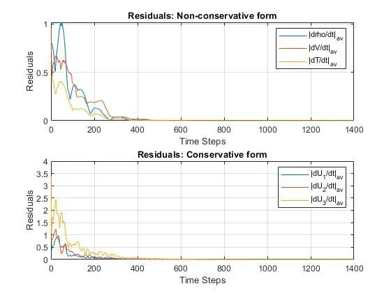
plot(1:nt,residual1)
grid on
xlabel('Time Steps')
ylabel('Residuals')
legend('|drho/dt|_{av}','|dV/dt|_{av}','|dT/dt|_{av}')
title('Residuals: Non-conservative form')
subplot(2,1,2)
plot(1:nt,residual2)
grid on
xlabel('Time Steps')
ylabel('Residuals'); yticks(0:0.5:4);
legend('|dU_1/dt|_{av}','|dU_2/dt|_{av}','|dU_3/dt|_{av}')
title('Residuals: Conservative form')

figure(5)
hold on; grid on;
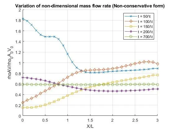
plot(x,m1(50,:),'-x')
plot(x,m1(100,:),'-d')
plot(x,m1(150,:),'-s')
plot(x,m1(200,:),'-*')
plot(x,m1(700,:),'-o')
xlabel('X/L')
ylabel('rhoAV/rho_0A_0V_0')
legend('t = 50/\t','t = 100/\t','t = 150/\t','t = 200/\t','t = 700/\t')
title('Variation of non-dimensional mass flow rate (Non-conservative form)')

figure(6)
hold on; grid on;
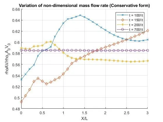
plot(x,m2(100,:),'-x')
plot(x,m2(150,:),'-d')
plot(x,m2(200,:),'-*')
plot(x,m2(700,:),'-o')
xlabel('X/L')
ylabel('rhoAV/rho_0A_0V_0')
legend('t = 100/\t','t = 150/\t','t = 200/\t','t = 700/\t')
title('Variation of non-dimensional mass flow rate (Conservative form)')

figure(7)
hold on; grid on;
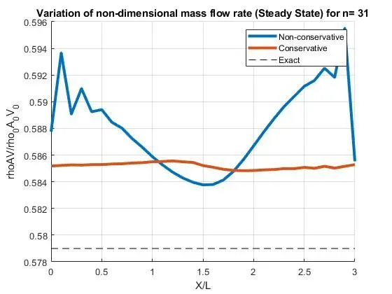
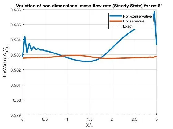
plot(x,m1(end,:),'LineWidth',3)
plot(x,m2(end,:),'LineWidth',3)
plot(x,0.579*ones(length(x),1),'--k')
xlabel('X/L')
ylabel('rhoAV/rho_0A_0V_0')
legend('Non-conservative','Conservative','Exact')
title('Variation of non-dimensional mass flow rate (Steady State) for n= 61')
CONSERVATIVE FUNCTION
function [p, t, v, P, m, M, p_t, t_t, v_t, P_t, M_t, residual]= consevative(x,dx,nt,gamma,a,c)

% initial conditions

for i =1:length(x)
if x(i)>=0 && x(i)<0.5
    p_o(i) = 1;
    t_o(i)=1;
elseif x(i)>= 0.5 && x(i)< 1.5
    p_o(i)= 1.0 - 0.366*(x(i)-0.5);
    t_o(i)= 1.0 - 0.167*(x(i)-0.5);

elseif x(i)>= 1.5 && x(i)<= 3.5
    p_o(i)= 0.634 - 0.3879*(x(i)-1.5);
    t_o(i)= 0.833 - 0.3507*(x(i)-1.5);
end
% v_o(i)= 0.59/p_o(i)*a(i);
end
v_o= 0.59./(p_o.*a);
throat= find(a==1);
p=p_o;
t=t_o;
v=v_o;
P= p.*t;
%m = zeros(nt,length(x));
U1= p.*a;
U2= p.*a.*v;
U3= p.*((t./(gamma-1)) + 0.5*(gamma)*v.^2).*a;

p_t = zeros(nt,1);
t_t = p_t;
v_t = t_t;
P_t = v_t;
M_t = P_t;
residual = zeros(nt,3);


% Time loop
for k= 1:nt
    U1_old= U1;
    U2_old= U2;
    U3_old= U3;
    dt = min( c*dx./(t.^0.5 + v));

    F1= U2;
    F2 = (U2.^2)./U1+((gamma-1)/gamma)*(U3 - 0.5*gamma*(U2.^2)./U1);
    F3 = gamma*U2.*U3./U1 - 0.5*gamma*(gamma-1)*(U2.^3)./(U1.^2);

    %predictor loop
    for i= 2:length(x)-1
        dF1dx= (F1(i+1) - F1(i))/dx;
        dF2dx= (F2(i+1) - F2(i))/dx;
        dF3dx= (F3(i+1) - F3(i))/dx;
        %dlogdx= (log(a(i+1)) - log(a(i)))/dx;
        dAdx = (a(i+1) - a(i))/dx;
        %J2= (gamma-1)./gamma.*(U3 - 0.5*gamma*(U2.^2./U1)).*dlogdx;
        J2 = (1/gamma)*p(i)*t(i)*dAdx;
        % continuity equation
        dU1dt_p(i)= -dF1dx;
        % momentum equation
        dU2dt_p(i)= -dF2dx + J2;
        % Energy equation
        dU3dt_p(i)= -dF3dx;

        % solution update
        U1(i) = U1(i) + dU1dt_p(i)*dt;
        U2(i) = U2(i) + dU2dt_p(i)*dt;
        U3(i) = U3(i) + dU3dt_p(i)*dt;

    end
    p = U1./a;
    v = U2./U1;
    t = (gamma-1)*((U3./U1) - 0.5*gamma*v.^2);
    F1= U2;
    F2 = (U2.^2)./U1+((gamma-1)/gamma)*(U3 - 0.5*gamma*(U2.^2)./U1);
    F3 = gamma*U2.*U3./U1 - 0.5*gamma*(gamma-1)*(U2.^3)./(U1.^2);

    % correction loop
    for i= 2:length(x)-1
        dF1dx= (F1(i) - F1(i-1))/dx;
        dF2dx= (F2(i) - F2(i-1))/dx;
        dF3dx= (F3(i) - F3(i-1))/dx;
        %dlogdx= (log(a(i+1)) - log(a(i)))/dx;
        %J2= (gamma-1)./gamma.*(U3 - 0.5*gamma*(U2.^2/U1)).*dlogdx;
        dAdx = (a(i) - a(i-1))/dx;
        J2 = (1/gamma)*p(i)*t(i)*dAdx;
        % continuity equation
        dU1dt_c(i)= -dF1dx;
        % momentum equation
        dU2dt_c(i)= -dF2dx + J2;
        % Energy equation
        dU3dt_c(i)= -dF3dx;
    end

    % average of corrector & predictor
        dU1dt = 0.5*(dU1dt_p + dU1dt_c);
        dU2dt = 0.5*(dU2dt_p + dU2dt_c);
        dU3dt = 0.5*(dU3dt_p + dU3dt_c);
        residual(k,1) = max(abs(dU1dt));
        residual(k,2) = max(abs(dU2dt));
        residual(k,3) = max(abs(dU3dt));

        % final solution update
        for i=2:length(x)-1
            U1(i) = U1_old(i) + dU1dt(i)*dt;
            U2(i) = U2_old(i) + dU2dt(i)*dt;
            U3(i) = U3_old(i) + dU3dt(i)*dt;
        end
        % Boundary conditions
        U1(1) = p(1)*a(1);
        U1(end) = 2*U1(end-1) - U1(end-2);
        U2(1) = 2*U2(2) - U2(3);
        U2(end) = 2*U2(end-1) - U2(end-2);

        U3(1) = U1(1)*((t(1)/(gamma-1)) + 0.5*gamma*v(1)^2);
        U3(end) = 2*U3(end-1) - U3(end-2);

        p= U1./a;
        v = U2./U1;
        t = (gamma-1)*((U3./U1) - 0.5*gamma*v.^2);
        M = v./(t.^0.5);
        P = p.*t;
        m(k,:) = p.*a.*v;
        p_t(k) = p(throat);
        v_t(k) = v(throat);
        t_t(k) = t(throat);
        P_t(k) = P(throat);
        M_t(k) = M(throat);
end

end
NON-CONSERVATIVE FUNCTION
function [p, t, v, P, m, M, p_t, t_t, v_t, P_t, M_t, residual] = non_conservative(x,dx,nt,gamma,a,c)

 % Calculate intial profiles
 p_o= 1- 0.3146*x;
 t_o= 1- 0.2314*x;
 v_o=(0.1 + 1.09*x).*t_o.^0.5;
 p=p_o;
 t=t_o;
 v=v_o;
throat= find(a==1);
m = zeros(nt,length(x));
p_t = zeros(nt,1);
t_t = p_t;
v_t = t_t;
P_t = v_t;
M_t = P_t;
residual = zeros(nt,3);


  for k= 1:nt

     p_old=p;
     v_old=v;
     t_old=t;
     dt = min(c*dx./(t.^0.5 + v));

     %Predictor method
     for i= 2:length(x)-1
         dvdx= (v(i+1) - v(i))/dx;
         dpdx= (p(i+1) - p(i))/dx;
         dxlog= (log(a(i+1)) - log(a(i)))/dx;
         dtdx= (t(i+1) -t(i))/dx;

         % continuity equation
         dpdt_p(i)= - p(i)*dvdx - p(i)*v(i)*dxlog - v(i)*dpdx;

         % momentum equation
         dvdt_p(i)= - v(i)*dvdx - (1/gamma)*(dtdx + (t(i)/p(i))*dpdx);

         %energy equation
         dtdt_p(i)= - v(i)*dtdx - (gamma-1)*t(i)*(dvdx + (v(i))*dxlog);

         %solution update
         p(i)= p(i) + dpdt_p(i)*dt;
         v(i)= v(i) + dvdt_p(i)*dt;
         t(i)= t(i) + dtdt_p(i)*dt;
     end

         %corector method
     for i= 2:length(x)-1
         dvdx= (v(i) - v(i-1))/dx;
         dpdx= (p(i) - p(i-1))/dx;
         dxlog= (log(a(i)) - log(a(i-1)))/dx;
         dtdx= (t(i) -t(i-1))/dx;

         % continuity equation
         dpdt_c(i)= - p(i)*dvdx - p(i)*v(i)*dxlog - v(i)*dpdx;

         % momentum equation
         dvdt_c(i)= - v(i)*dvdx - (1/gamma)*(dtdx + (t(i)/p(i))*dpdx);

         %energy equation
         dtdt_c(i)= - v(i)*dtdx - (gamma-1)*t(i)*(dvdx + (v(i))*dxlog);

     end

     % compute average
     dpdt= 0.5*(dpdt_p + dpdt_c);
     dvdt= 0.5*(dvdt_p + dvdt_c);
     dtdt= 0.5*(dtdt_p + dtdt_c);
     residual(k,1) = max(abs(dpdt));
     residual(k,2) = max(abs(dvdt));
     residual(k,3) = max(abs(dtdt));

     % final update
     for i= 2:length(x)-1
     p(i) = p_old(i) + dpdt(i)*dt;
     v(i) = v_old(i) + dvdt(i)*dt;
     t(i) = t_old(i) + dtdt(i)*dt;
     end


     % apply boundary conditions
     %inlet & outlet conditions
        p(end) = 2*p(end-1)-p(end-2);
        v(1) = 2*v(2)-v(3);
        v(end) = 2*v(end-1)-v(end-2);
        t(end) = 2*t(end-1)-t(end-2);
        % final updates
        M = v./(t.^0.5);
        P = p.*t;
        m(k,:) = p.*a.*v;
        p_t(k) = p(throat);
        v_t(k) = v(throat);
        t_t(k) = t(throat);
        P_t(k) = P(throat);
        M_t(k) = M(throat);
  end


end
RESULTS
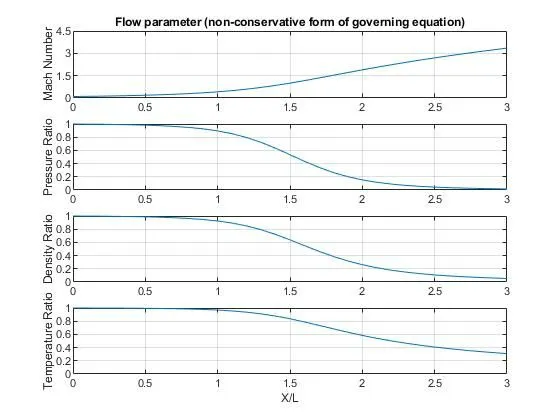
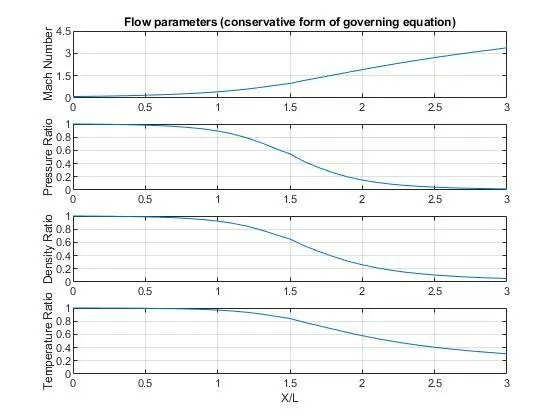
CONCLUSIONS
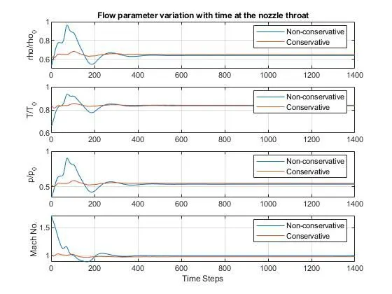
- Comparing the conservative and non-conservative form the values of the flow variables at the throat of nozzle are plotted at each time step. It can be observed th at smaller time steps, The behaviour of non-conservative forms shows unstable results.But with increase in time step the difference is conservative and non conservative diminishes.
- If we notice the residuals of both approaches the conservative form converges to steady faster than non- conservative.
- There is appreciable difference in how the mass flow rate varies with time step but it can be observed that at time step of 700 delta t the mass flow becomes constant. The conservative form produces an almost constant mass flow but non-conservative has highly fluctuating mass flow.
- On varying the grid size it is noted that the conservative form almost maintains its consistency but non- conservative becomes stable on the increasing grid size.
- Maccormack provides stable and close exact solutions So, its widely implemented to solve varioous flow problems.