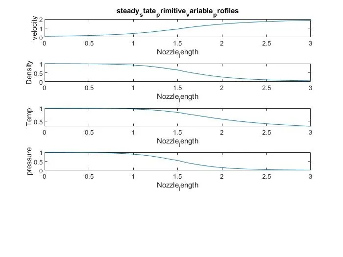
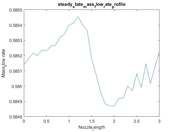
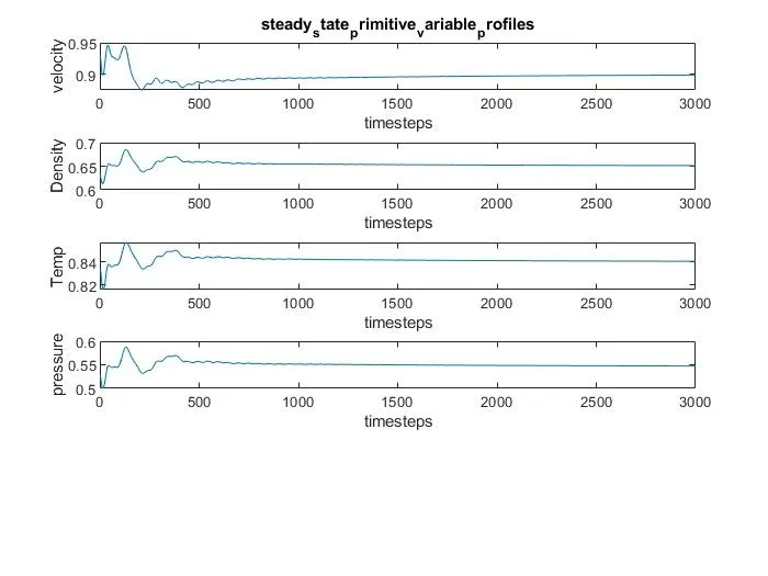
Week 7 - Simulation of a 1D Super-sonic nozzle flow simulation using Macormack Method
AIM: To simulate the isentropic flow through a quasi 1D subsonic-supersonic nozzle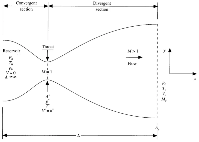
We consider steady, isentropic flow through convergent_Divergent nozzle.The flow at the inlet comes from the reservoir where the pressure, temp are denoted by p0,T0 respectively.The cross_sectional area of the reservoir is large (theroticallyA=infinity) & where velocity is less ,The flow Expands isentropically to supersonic speeds at the nozzle exit,where exit preesures ,temp,velocity,&Mach number denoted by Pe,Te, Ve & Me respectively .The flow is locally subsonic in the convergent of the nozzle,sonic at the throat (minimum area)& super_sonic at the divergent section The sonic flow (M=1) at the throat means that the local velocity at this section is equal to the local speed of sound.
The area of sonic Throat is denoted by a*,we assume that a any given section,where the cross_sectional area "a" the flow properties are uniform across the cross section although the area is afunction of distance along the nozzle 'x'and therefore in reality the flow is two _dimensional(the flow varies in the two _directional in xy space
The governing continuity ,momentum,and energy equations for this Quasi_one dimensional,steady,isentropic flow can be expressed, respectively
Continuity eq:
- rho1*V1*A1=rho2*V2*A2
Momentum Eq:
- P1A1+rho1*V1^2*A1+Integral p*dA= P2A2+rho2*V2^2*A2
Energy Eq:
- h1+v1^2/2=h2+V2^2
The Mach number variation through the nozzle is governed by the area ratio A/A* through the relation
- (A/A*)^2= 1/M^2[2/gamma+1(1+gamma-1/2*M^2)]^(gamma+1)*(gamma-1)
where,
- gamma=cp/cv
- The governing Equations will be couched in terms of partial differntial equations suitable for Time_marching solution of Quasi-one dimensional flow. the finite difference expressions pertaining to Maccormacks technique as applied to this problem.
- The nozzle flow just described above just does not happen by itself,it takes a force to acclerate a given mass ,the force exerted on the gas to acclerate it through the nozzle is supplied by the pressure ratio across the nozzle ,p0/pe for a nozzle with specified area ratio Ae/A.
- The application of Maccormack 's technique In particular, we will set up a time-marching for the quasi-one-dimensional nozzle flow.
- Note that, in reality, the real nozzle flow is a two-dimensional flow because, with tharea changing as a function of x, in actuality there will be flow-field variations inboth the x and y directions. This is the real physics of the flow,assumption of quasi-one-dimensional flow dictates that the flow properties arefunctions of x only.
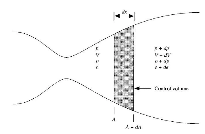
- This controlvolume 1s a slice of the nozzle flow, where the infinitesimal thickness of the slice is~x. On the left side of the control volume, consistent with the quasi-one-dimensional assumption, _the density, :elocity, pressure, and internal energy, denoted by p,V, p, and e, respectively, are umform over the area A. Similarly, on the right side ofthe control volume, the density, velocity, pressure, and internal energy, denoted byP + dp, V + dV, p + dp, and e + de, respectively, are uniform over the area(A+dA).
Non_conservative form of Eq:



Conservative Form:
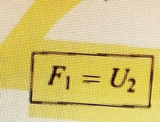
%%NON__conservative FORM

 clc
 clear all
 close all
 %inputs
 %x__array(1dimensional)
 n=31;
 x=linspace(0,3,n);
 dx=x(2)-x(1);
 gamma=1.4;

 %calculate___ initial profiles
 rho=1-0.3146*x;
 t=1-0.2314*x;
 v=(0.1+1.09*x).*t.^0.5;
 a=1+2.2*(x-1.5).^2;

 %Time___steps
 nt=1400;
 CFL = 0.8;


%Time__Loop
 for k=1:nt

 % CFL = (u+a).dt/dx
 % a = sqrt(gamma*R*T)

  dt(k) = min((CFL*dx)./(v+sqrt(t)));

 % Copying initial time step values
  rho_old=rho;
  v_old=v;
  t_old=t;


  %predictor__step
  %continuity___ eq

   for j=2:n-1
      %drho_dt_p=-rho(j)*(v(j+1)-v(j))/dx-rho(j)*v(j)*(log(a(j+1)-log(a(j))))/dx-v(j)*(rho(j+1)-rho(j))/dx
      dv_dx      =(v(j+1)-v(j))/dx;
      drho_dx    =(rho(j+1)-rho(j))/dx;
      dlog_a_dx  = (log(a(j+1))-log(a(j)))/dx;
      dt_dx      =(t(j+1)-t(j))/dx;

      %continuity__ eq:
      drho_dt_p(j)=-rho(j)*dv_dx-rho(j)*v(j)*dlog_a_dx-v(j)*drho_dx;

      %Momentum ___eq:
      dv_dt_p(j)=-v(j)*dv_dx-(1/gamma)*(dt_dx+(t(j)/rho(j))*drho_dx);

      %Energy __eq:
      dt_dt_p(j)=-v(j)*dt_dx-(gamma-1)*t(j)*(dv_dx+v(j)*dlog_a_dx);

   % solution__update

      rho(j) = rho(j) +drho_dt_p(j)*dt(k);
      v(j)   =   v(j) +dv_dt_p(j)*dt(k);
      t(j)   =  t(j)  +dt_dt_p(j)*dt(k);
   end


   %corrected__method
   for j=2:n-1
      %drho_dt_p=-rho(j)*(v(j+1)-v(j))/dx-rho(j)*v(j)*(log(a(j+1)-log(a(j))))/dx-v(j)*(rho(j+1)-rho(j))/dx
      dv_dx= (v(j)-v(j-1))/dx;

      drho_dx=(rho(j)-rho(j-1))/dx;

      dlog_a_dx= (log(a(j))-log(a(j-1)))/dx;

      dt_dx=(t(j)-t(j-1))/dx;

      %continuity__ eq:
       drho_dt_c(j)=-rho(j)*dv_dx-rho(j)*v(j)*dlog_a_dx-v(j)*drho_dx;

      %Momentum ___eq:
       dv_dt_c(j)=-v(j)*dv_dx-(1/gamma)*(dt_dx+(t(j)/rho(j))*drho_dx);

      %Energy __eq:
       dt_dt_c(j)=-v(j)*dt_dx-(gamma-1)*t(j)*(dv_dx+v(j)*dlog_a_dx);

    end

  %compute__avg__ time derivative
   drho_dt =0.5*(drho_dt_p+drho_dt_c);

   dv_dt =0.5*(dv_dt_p+dv_dt_c);


   dt_dt =0.5*(dt_dt_p+dt_dt_c);

  %final_solution_update

  for i=2:n-1
    rho(i) =rho_old(i) + drho_dt(i)*dt(k);
    v(i) =v_old(i) + dv_dt(i)*dt(k);
    t(i)=t_old(i) + dt_dt(i)*dt(k);
  end

%Apply_boundary_conditions
%Inlet
  rho(1)=1;
  v(1)=2*v(2)-v(3);
  t(1)=1;

 %Outlet
   rho(n)=2*rho(n-1)-rho(n-2);
   v(n)=2*v(n-1)-v(n-2);
   t(n)=2*t(n-1)-t(n-2);

  % pressure
  p=rho.*t

  % Mach number
   M = v./sqrt(t)
  % Mass flow rate
  m = rho.*a.*v;

  rho_th(k) = rho(16);
    v_th(k) = v(16);
    t_th(k) = t(16);
    p_th(k) = p(16);


 end


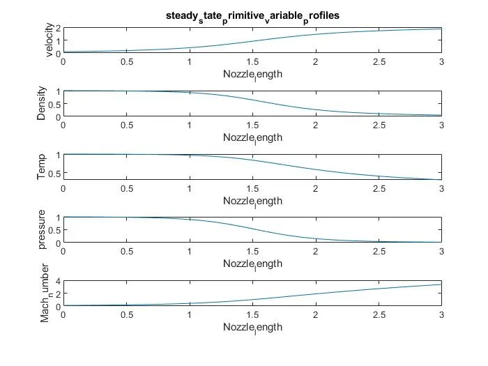
figure(1)
subplot(5,1,1)
plot(x,v);
xlabel('Nozzle_length');
ylabel('velocity');
title('steady_state_primitive_variable_profiles');
subplot(5,1,2);
plot(x,rho);
xlabel('Nozzle_length');
ylabel('Density');
subplot(5,1,3);
plot(x,t);
xlabel('Nozzle_length');
ylabel('Temp');
subplot(5,1,4);
plot(x,p);
xlabel('Nozzle_length');
ylabel('pressure');
subplot(5,1,5);
plot(x,M);
xlabel('Nozzle_length');
ylabel('Mach_number')

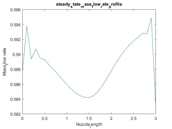
figure(2)
plot(x,m);
xlabel('Nozzle_length');
ylabel('Mass_flow rate');
title('steady_state_mass_flow_rate_profile')

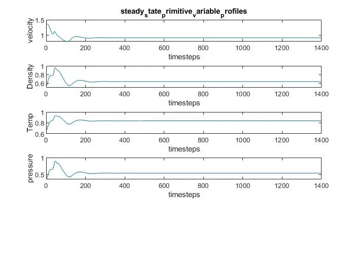
figure(3)
subplot(5,1,1)
plot(v_th);
xlabel('timesteps');
ylabel('velocity');
title('steady_state_primitive_variable_profiles');
subplot(5,1,2);
plot(rho_th);
xlabel('timesteps');
ylabel('Density');
subplot(5,1,3);
plot(t_th);
xlabel('timesteps');
ylabel('Temp');
subplot(5,1,4);
plot(p_th);
xlabel('timesteps');
ylabel('pressure');
%%Conservative__Form

close all
clear all
clc

% Inputs

n = 31;
x = linspace(0,3,n);
dx = x(2)-x(1) ;
gamma = 1.4;
CFL = 0.4;
nt = 3000;


% Initial Conditions

a = 1+2.2*(x-1.5).^2;


% Initial___Conditions
for i=1:1:length(x)

    if(x(i)>=0 && x(i)<=0.5)
        rho(i)=1;
        t(i)=1;

    elseif (x(i)>=0.5  && x(i)<=1.5)
          rho(i)=1-0.366*(x(i)-0.5);
          t(i)=1-0.167*(x(i)-0.5);

    elseif (x(i)>=1.5  && x(i)<=3)
           rho(i)= 0.634-0.3879*(x(i)-1.5);
           t(i)= 0.833-0.3507*(x(i)-1.5);

    end
end

% Solution Vectors

V = 0.59./(rho.*a);
U1= rho.*a;
U2= rho.*a.*V;
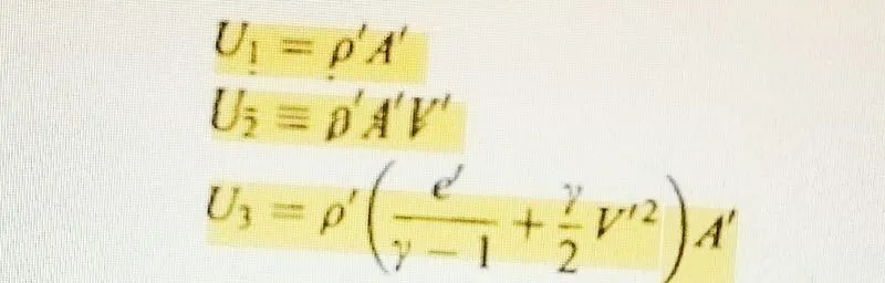
U3= rho.*a.*((t./(gamma-1))+(gamma/2).*V.^2);


% Solution Vectors
% Time ____loop
for tt = 1:1:(nt)
 % Storing Initial Values
    U1_old = U1;
    U2_old = U2;
    U3_old = U3;

    dt =min((CFL.*dx)./(t.^(0.5)+V));

    F1= U2;
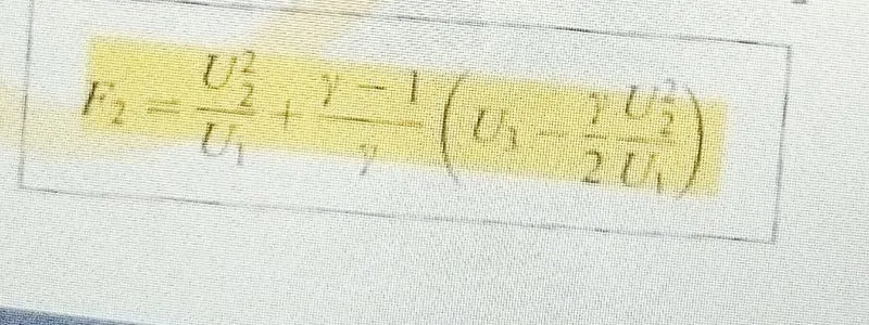
    F2= ((U2.^2)./U1 )+ ((gamma-1)/gamma).*(U3-((gamma/2) * (U2.^2)./U1));
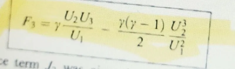
    F3= ((gamma*U2.*U3)./U1) - ((gamma*(gamma-1)/2) * (U2.^3)./(U1.^2));

    for nx = 2:n-1
    % Predictors___ step
      % Source term J2
      J2(nx) = (1/gamma)*rho(nx)*t(nx)*((a(nx+1)-a(nx))/dx);
      % Predictors___ Step__ derivative
      du1dt_p(nx) = -(F1(nx+1)-F1(nx))./dx ;
      du2dt_p(nx) = -(F2(nx+1)-F2(nx))./dx + J2(nx) ;
      du3dt_p(nx) = -(F3(nx+1)-F3(nx))./dx ;

      % Solution___ update
      U1(nx) = U1(nx) + du1dt_p(nx).*dt;
      U2(nx) = U2(nx) + du2dt_p(nx).*dt;
      U3(nx) = U3(nx) + du3dt_p(nx).*dt;

    end
    rho =U1./a ;
    V=U2./U1;
    t = (gamma-1).*((U3./U1) - (gamma./2).*(V).^2);

    % correctors___step
    % Flux Vector
    F1= U2;
    F2= ((U2.^2)./U1 )+ ((gamma-1)/gamma).*(U3-((gamma/2) * (U2.^2)./U1));
    F3= ((gamma*U2.*U3)./U1) - ((gamma*(gamma-1)/2) * (U2.^3)./(U1.^2));


    for j = 2:n-1
    % Source term J2
    J2(j) = (1/gamma)*rho(j)*t(j)*((a(j)-a(j-1))/dx);
    % Correctors Step derivative
    du1dt_c(j) = -(F1(j)-F1(j-1))./dx ;
    du2dt_c(j) = -(F2(j)-F2(j-1))./dx + J2(j) ;
    du3dt_c(j) = -(F3(j)-F3(j-1))./dx ;

    end

    % Average time derivative
    du1dt_avg = 0.5.*(du1dt_p + du1dt_c);
    du2dt_avg = 0.5.*(du2dt_p + du2dt_c);
    du3dt_avg = 0.5.*(du3dt_p + du3dt_c);

    % Final Solution update
    for y =2:n-1

        U1(y) = U1_old(y) + du1dt_avg(y).*dt;
        U2(y) = U2_old(y) + du2dt_avg(y).*dt;
        U3(y) = U3_old(y) + du3dt_avg(y).*dt;

    end

% Apply___ Boundary Conditions
% Inlet___


    U1(1) = rho(1).*a(1);
    U2(1)= 2*U2(2)-U2(3);
    U3(1)= U1(1)*((t(1)/(gamma-1))+(gamma/2)*V(1).^2);
 %Outlet___
    U1(n)= 2*U1(n-1)- U1(n-2);
    U2(n)= 2*U2(n-1)- U2(n-2);
    U3(n)= 2*U3(n-1)- U3(n-2);

    % calcultaing___ primitive variables
    rho = U1./a;
    V= U2./U1;
    t = (gamma-1)*((U3./U1)-(gamma/2)*V.^2);
    m = U2;
    p= rho.*t;

    rho_th(tt) = rho(16);
    V_th(tt) = V(16);
    t_th(tt) = t(16);
    p_th(tt) = p(16);


end


figure(1)
subplot(5,1,1)
plot(x,V);
xlabel('Nozzle_length');
ylabel('velocity');
title('steady_state_primitive_variable_profiles');
subplot(5,1,2);
plot(x,rho);
xlabel('Nozzle_length');
ylabel('Density');
subplot(5,1,3);
plot(x,t);
xlabel('Nozzle_length');
ylabel('Temp');
subplot(5,1,4);
plot(x,p);
xlabel('Nozzle_length');
ylabel('pressure');

figure(2)
plot(x,m);
xlabel('Nozzle_length');
ylabel('Mass_flow rate');
title('steady_state_mass_flow_rate_profile')

figure(3)
subplot(5,1,1)
plot(V_th);
xlabel('timesteps');
ylabel('velocity');
title('steady_state_primitive_variable_profiles');
subplot(5,1,2);
plot(rho_th);
xlabel('timesteps');
ylabel('Density');
subplot(5,1,3);
plot(t_th);
xlabel('timesteps');
ylabel('Temp');
subplot(5,1,4);
plot(p_th);
xlabel('timesteps');
ylabel('pressure');