Week 7 - Simulation of a 1D Super-sonic nozzle flow simulation using Macormack Method
Program:
%Main program

clear all
close all
clc

% Domain initialization

L=3;
nx=31;
x=linspace(0,L,nx);
dx=x(2)-x(1);
C=0.5;
nt=1400;
gamma=1.4;

%Nozzle area

A=1+2.2*(x-1.5).^2;

%Computing the flow variable through conservative and non-conservative
%forms

[rho1, V1, T1, p1, M1, m1, rho_t1, V_t1, p_t1, T_t1, M_t1, residual1] = non_conservative_sh(x, dx, A, C, nt, gamma);
[rho2, V2, T2, p2, M2, m2, rho_t2, V_t2, p_t2, T_t2, M_t2, residual2] = conservative_sh(x, dx, A, C, nt, gamma);

%Plotting of results

figure(1)
subplot(4,1,1)
plot(x,M1)
grid on; ylim([0 4.5]); yticks(0:1.5:4.5);
ylabel('Mach Number')
title('Flow parameter (non-conservative form of governing equation)')
subplot(4,1,2)
plot(x,p1)
grid on; yticks(0:0.2:1);
ylabel('Pressure ratio')
subplot(4,1,3)
plot(x,rho1)
grid on; yticks(0:0.2:1);
ylabel('Density Ratio')
subplot(4,1,4)
plot(x,T1)
grid on; ylim([0 1]); yticks(0:0.2:1);
ylabel('Temperature Ratio')
xlabel('X/L')

figure(2)
subplot(4,1,1)
plot(x,M2)
grid on; ylim([0 4.5]); yticks(0:1.5:4.5);
ylabel('Mach Number')
title('Flow parameter (conservative form of governing equation)')
subplot(4,1,2)
plot(x,p2)
grid on; yticks(0:0.2:1);
ylabel('Pressure ratio')
subplot(4,1,3)
plot(x,rho2)
grid on; yticks(0:0.2:1);
ylabel('Density Ratio')
subplot(4,1,4)
plot(x,T2)
grid on; ylim([0 1]); yticks(0:0.2:1);
ylabel('Temperature Ratio')
xlabel('X/L')

figure(3)
subplot(4,1,1)
plot(1:nt,rho_t1)
hold on
plot(1:nt,rho_t2)
grid on; ylim([0 1]); yticks(0:0.2:1);
ylabel('rho/rho_0')
title('Flow parameter variation with time at the nozzle throat');
legend('Non-conservative', 'Conservative');
subplot(4,1,2)
plot(1:nt,T_t1)
hold on
plot(1:nt,T_t2)
grid on; yticks(0:0.2:1);
ylabel('T/T_0')
legend('Non-conservative', 'Conservative');
subplot(4,1,3)
plot(1:nt, p_t1)
hold on
plot(1:nt,p_t2)
grid on; yticks(0:0.2:1);
ylabel('p/p_0')
legend('Non-conservative', 'Conservative');
subplot(4,1,4)
plot(1:nt,M_t1)
hold on
plot(1:nt, M_t2)
grid on; yticks(0:0.2:2);
ylabel('Mach No.')
xlabel('Time steps')
legend('Non-conservative', 'Conservative');

figure(4)
subplot(2,1,1)
plot(1:nt,residual1)
grid on
xlabel('Time Steps')
ylabel('Residuals')
legend('|drho/dt|_{av}', '|dV/dt|_{av}', '|dT/dt|_{av}')
title('Residuals: Non-conservative form')
subplot(2,1,2)
plot(1:nt,residual2)
grid on
xlabel('Time steps')
ylabel('Residuals'); yticks(0:0.5:4);
legend('|dU_1/dt|_{av}', '|dU_2/dt|_{av}', '|dU_3/dt|_{av}')
title('Residuals: Conservative form')

figure(5)
hold on; grid on;
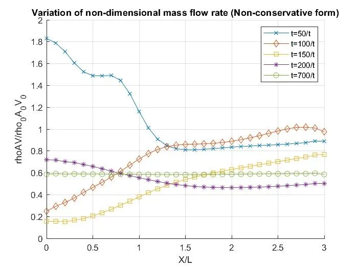
plot(x,m1(50,:),'-x')
plot(x,m1(100,:),'-d')
plot(x,m1(150,:),'-s')
plot(x,m1(200,:),'-*')
plot(x,m1(700,:),'-o')
xlabel('X/L')
ylabel('rhoAV/rho_0A_0V_0')
legend('t=50/t', 't=100/t', 't=150/t', 't=200/t', 't=700/t' )
title('Variation of non-dimensional mass flow rate (Non-conservative form)')

figure(6)
hold on; grid on;
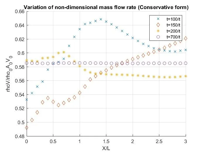
plot(x,m2(100,:), 'x')
plot(x,m2(150,:), 'd')
plot(x,m2(200,:), '*')
plot(x,m2(700,:), 'o')
xlabel('X/L')
ylabel('rhoV/rho_0A_0V_0')
legend('t=100/t', 't=150/t', 't=200/t', 't=700/t' )
title('Variation of non-dimensional mass flow rate (Conservative form)')

figure(7)
hold on; grid on;
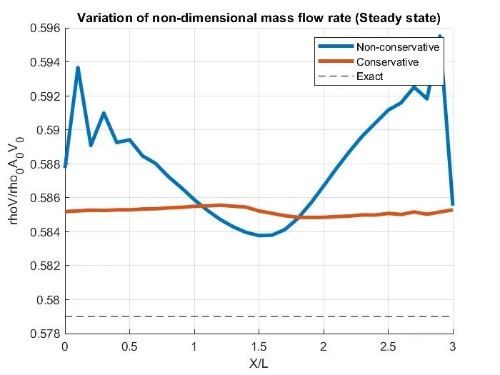
plot(x,m1(end,:), 'Linewidth', 3)
plot(x,m2(end,:), 'Linewidth', 3)
plot(x,0.579*ones(length(x),1),'--k')
xlabel('X/L')
ylabel('rhoV/rho_0A_0V_0')
legend('Non-conservative', 'Conservative', 'Exact')
title('Variation of non-dimensional mass flow rate (Steady state)')


% Solver for conservative form of governing equation

function [rho2, V2, T2, p2, M2, m2, rho_t2, V_t2, p_t2, T_t2, M_t2, residual2] = conservative_sh(x, dx, A, C, nt, gamma)

%Initial conditions

rho_0=zeros(1,length(x));
T_0=rho_0;
V_0=T_0;
for i=1:length(x)
    if x(i)>=0 && x(i)<0.5
        rho_0(i)=1;
         T_0(i)=1;

    elseif x(i)>=0.5 && x(i)<1.5
        rho_0(i)=1-0.366*(x(i)-0.5);
        T_0(i)=1-0.167*(x(i)-0.5);

    elseif x(i)>=1.5 && x(i)<=3
        rho_0(i)=0.634-0.3879*(x(i)-1.5);
        T_0(i)=0.833-0.3507*(x(i)-1.5);
    end
    V_0(i)=0.59/(rho_0(i)*A(i));
end

throat=find(A==1);
rho=rho_0;
T=T_0;
V=V_0;
m=zeros(nt,length(x));
U1=rho.*A;
U2=rho.*A.*V;
U3=rho.*(T./(gamma-1)+(0.5*gamma)*(V.^2)).*A;
rho_t=zeros(nt,1);
T_t=rho_t;
V_t=T_t;
p_t=V_t;
M_t=p_t;
residual=zeros(nt,3);
for k=1:nt
    U1_old=U1;
    U2_old=U2;
    U3_old=U3;
    dt=min(C*dx./(T.^0.5+V));
    F1=U2;
    F2=(U2.^2)./U1+(gamma-1)/(gamma)*(U3-0.5*gamma*(U2.^2)./U1);
    F3=gamma*U2.*U3./U1-0.5*gamma*(gamma-1)*(U2.^3)./(U1.^2);

    % Predictor Loop
    for i=2:length(x)-1
        dF1dx=(F1(i+1)-F1(i))/dx;
        dF2dx=(F2(i+1)-F2(i))/dx;
        dF3dx=(F3(i+1)-F3(i))/dx;
        dAdx=(A(i+1)-A(i))/dx;
        J2=(1/gamma)*rho(i)*T(i)*dAdx;

        dU1dt_p(i)=-dF1dx;
        dU2dt_p(i)=-dF2dx+J2;
        dU3dt_p(i)=-dF3dx;

        % Intermediate update
        U1(i)=U1(i)+dU1dt_p(i)*dt;
        U2(i)=U2(i)+dU2dt_p(i)*dt;
        U3(i)=U3(i)+dU3dt_p(i)*dt;
    end
    rho=U1./A;
    V=U2./U1;
    T=(gamma-1)*((U3./U1)-0.5*gamma*V.^2);
    F1=U2;
    F2=((U2.^2)./U1)+(((gamma-1)/gamma)*(U3-((0.5*gamma)*(U2.^2)./U1)));
    F3=(gamma*((U2.*U3)./U1))-((0.5*gamma*(gamma-1))*((U2.^3)./U1.^2));

    % Corrector Loop
    for i=2:length(x)-1
        dF1dx=(F1(i)-F1(i-1))/dx;
        dF2dx=(F2(i)-F2(i-1))/dx;
        dF3dx=(F3(i)-F3(i-1))/dx;
        dAdx=(A(i)-A(i-1))/dx;
        J2=(1/gamma)*rho(i)*T(i)*dAdx;

        dU1dt_c(i)=-dF1dx;
        dU2dt_c(i)=-dF2dx+J2;
        dU3dt_c(i)=-dF3dx;
    end

    % Average of predictor and corrector step

    dU1dt=0.5*(dU1dt_p+dU1dt_c);
    dU2dt=0.5*(dU2dt_p+dU2dt_c);
    dU3dt=0.5*(dU3dt_p+dU3dt_c);

    residual(k,1)=max(abs(dU1dt));
    residual(k,2)=max(abs(dU2dt));
    residual(k,3)=max(abs(dU3dt));

    % Final solution update

    for i=2:length(x)-1
        U1(i)=U1_old(i)+dU1dt(i)*dt;
        U2(i)=U2_old(i)+dU2dt(i)*dt;
        U3(i)=U3_old(i)+dU3dt(i)*dt;
    end

    % Boundary Conditions
    U1(1)=rho(1)*A(1);
    U1(end)=2*U1(end-1)-U1(end-2);
    U2(1)=2*U2(2)-U2(3);
    U2(end)=2*U2(end-1)-U2(end-2);
    U3(1)=U1(1)*((T(1)/(gamma-1))+0.5*gamma*V(1)^2);
    U3(end)=2*U3(end-1)-U3(end-2);
    rho=U1./A;
    V=U2./U1;
    T=(gamma-1)*((U3./U1)-((0.5*gamma)*V.^2));
    M=V./(T.^0.5);
    p=rho.*T;
    m(k,:)=rho.*A.*V;
    rho_t(k)=rho(throat);
    V_t(k)=V(throat);
    T_t(k)=T(throat);
    p_t(k)=p(throat);
    M_t(k)=M(throat);
end
rho2=rho;
V2= V;
T2= T;
p2= p;
M2= M;
m2 = m;
rho_t2= rho_t;
V_t2= V_t;
p_t2= p_t;
T_t2= T_t;
M_t2= M_t;
residual2= residual;
end


% Solver for Non-conservative form of governing equation

function [rho1, V1, T1, p1, M1, m1, rho_t1, V_t1, p_t1, T_t1, M_t1, residual1] = non_conservative_sh(x, dx, A, C, nt, gamma)

%Initial conditions
rho_0 = 1 - 0.3146*x;
T_0 = 1- 0.2314*x;
V_0 = (0.1 + 1.09*x).*T_0.^0.5;
throat = find(A==1);
rho = rho_0;
T = T_0;
V = V_0;
m = zeros(nt,length(x));
rho_t = zeros(nt,1);
T_t = rho_t;
V_t = T_t;
p_t= V_t;
M_t = p_t;
residual = zeros(nt,3);
for k=1:nt
    rho_old = rho;
    T_old = T;
    V_old = V;
    dt = min(C*dx./(T.^0.5+V));

    %Predictor loop

    for i=2:length(x)-1
        dVdx= (V(i+1) - V(i))/dx;
        dlogAdx = (log(A(i+1)) - log(A(i)))/dx;
        drhodx = (rho(i+1) - rho(i))/dx;
        dTdx = (T(i+1) - T(i))/dx;

        drhodt_p(i) = -rho(i)*dVdx - rho(i)*V(i)*dlogAdx - V(i)*drhodx;
        dVdt_p(i) = -V(i)*dVdx - (1/gamma)*(dTdx + ((T(i)/rho(i))*drhodx));
        dTdt_p(i) = -V(i)*dTdx - (gamma-1)*T(i)*(dVdx +V(i)*dlogAdx);

        %Intermediate step

        rho(i) = rho(i) + drhodt_p(i)*dt;
        V(i) = V(i) + dVdt_p(i)*dt;
        T(i) = T(i) + dTdt_p(i)*dt;

    end

    % Corrector loop

    for i=2:length(x)-1
        dVdx = (V(i) - V(i-1))/dx;
        dlogAdx = (log(A(i)) - log(A(i-1)))/dx;
        drhodx = (rho(i) - rho(i-1))/dx;
        dTdx = (T(i) - T(i-1))/dx;

        drhodt_c(i) = -rho(i)*dVdx - rho(i)*V(i)*dlogAdx - V(i)*drhodx;
        dVdt_c(i) = -V(i)*dVdx - ((1/gamma)*(dTdx + ((T(i)/rho(i))*drhodx)));
        dTdt_c(i) = -V(i)*dTdx - (gamma-1)*T(i)*(dVdx + V(i)*dlogAdx);

    end

    %Average of predictor and corrector step

    drhodt = 0.5*(drhodt_p + drhodt_c);
    dVdt = 0.5*(dVdt_p + dVdt_c);
    dTdt = 0.5*(dTdt_p + dTdt_c);
    residual(k,1) = max(abs(drhodt));
    residual(k,2) = max(abs(dVdt));
    residual(k,3) = max(abs(dTdt));

    %FInal solution update

    for i=2:length(x) - 1
        rho(i) = rho_old(i) + drhodt(i)*dt;
        V(i) = V_old(i) + dVdt(i)*dt;
        T(i) = T_old(i) + dTdt(i)*dt;
    end

    %Boundary conditions
    rho(end) = 2*rho(end-1) - rho(end-2);
    V(1) = 2*V(2) - V(3);
    V(end) = 2*V(end-1) - V(end-2);
    T(end) = 2*T(end-1) - T(end-2);
    M = V./(T.^0.5);
    p = rho.*T;
    m(k,:) = rho.*A.*V;
    rho_t(k) = rho(throat);
    V_t(k) = V(throat);
    T_t(k) = T(throat);
    p_t(k) = p(throat);
    M_t(k) = M(throat);
end
rho1=rho;
V1= V;
T1= T;
p1= p;
M1= M;
m1 = m;
rho_t1= rho_t;
V_t1= V_t;
p_t1= p_t;
T_t1= T_t;
M_t1= M_t;
residual1= residual;
end
Theory:
Results:
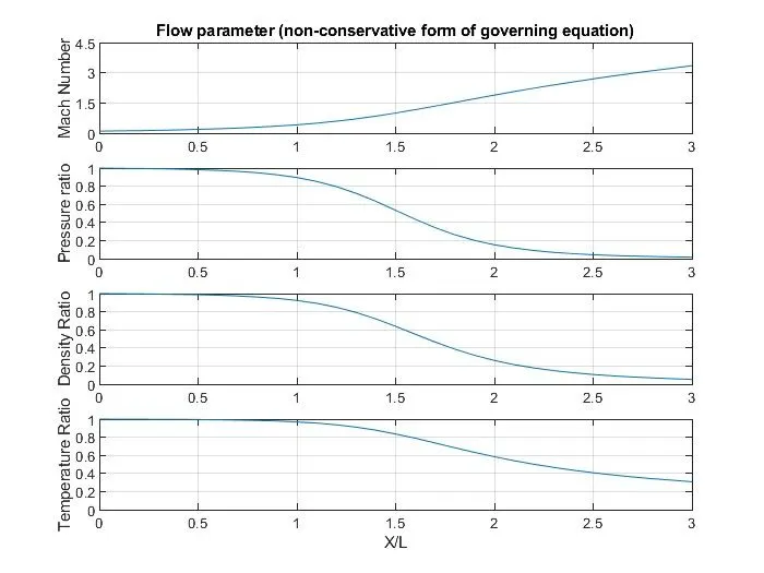
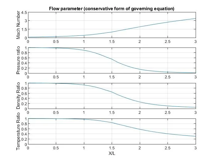
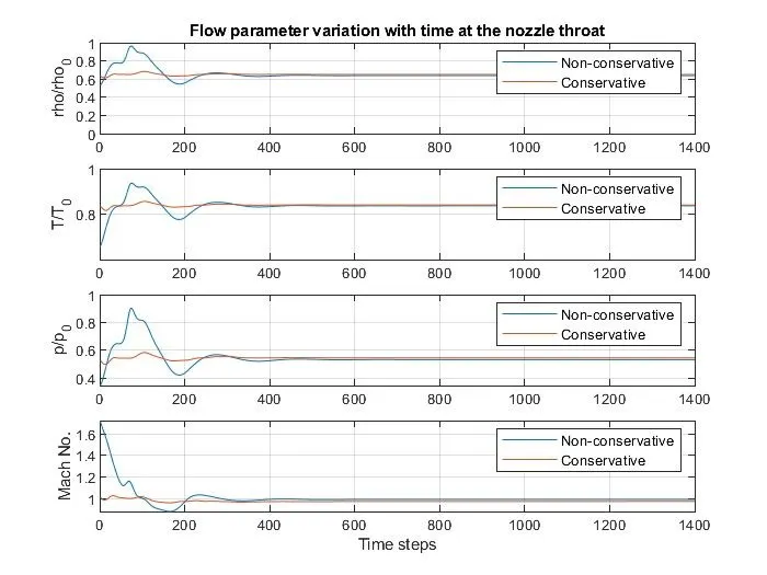
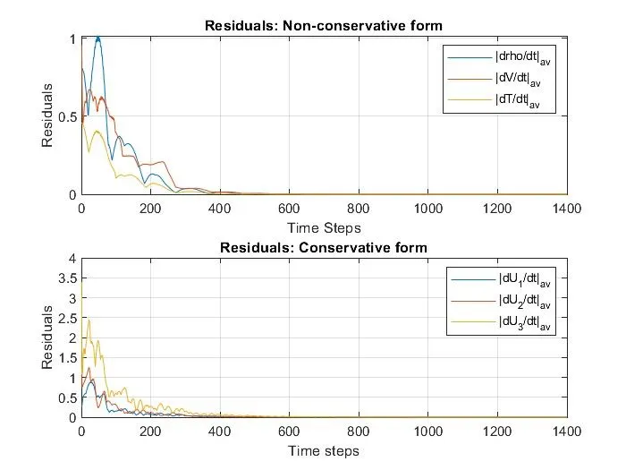
Theory:
We have considered a steady isentropic flow through a convergent-divergent nozzle.
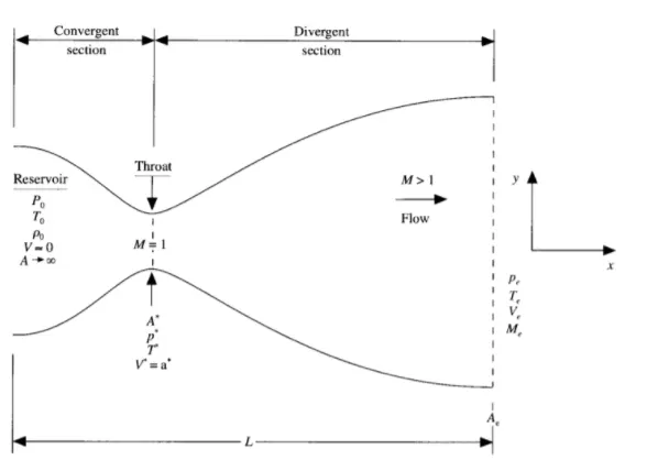
The flow to the inlet comes from a reservoir is large. Po and To are stagrnation pressure and temperature. In this case, the flow expands isentropically to supersonic speeds at the exit of the nozzle. The exit pressure, temperature and other conditions are denoted with a subscript 'e'.
Mackormack method setup -
In CFD, the Mackormack scheme is the most widely used discretization technique for obtaining solutions for hyperbolic partial differential equations.
It is an explicit method that gives second order accuracy without the involovement of second order derivative thus reducing the complexity of calculating it.
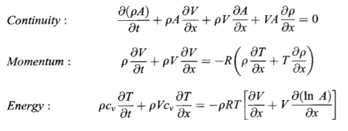
From the text book, we have considered the conservation equations to be,
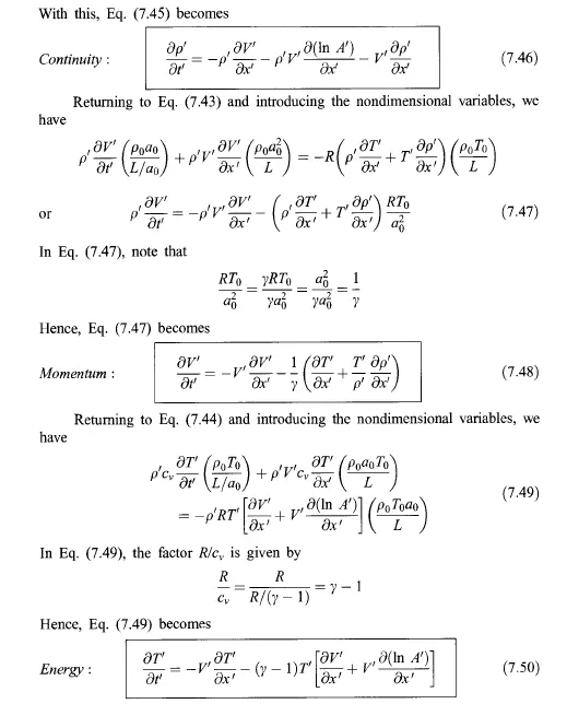
The reservoir temperature and density are denoted by T0 and `rho0` and we define non-dimensional temperature and density as `T' = T/(T0) and rho' = rho/(rho0)`with x'=x/L as the non-dimensional length.
After similar substitiution, we arrive at (image taken from the text)
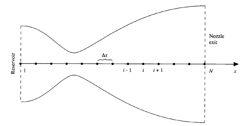
The FDM setup with the node points is as follows -
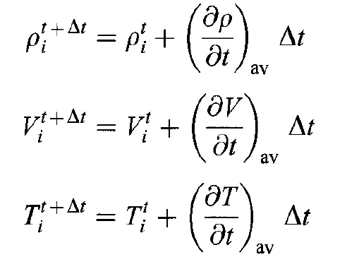
The flow field variables are as follows.
Calculation of time step -
where C, Courant number(Stability indicator) lesser than or eqaul to 1 for explicit case
Taking the grid point consideration for the 'i' th node,
For the 'i+1'th node,
Initial conditions are as follows -
The further process for solving can be inferred from the program.