Week 5.1 - Mid term project - Solving the steady and unsteady 2D heat conduction problem
Governing equation for heat conduction in two dimension is:
`(delT)/(delt) = alpha {(del^2T)/(del^2x)+(del^2T)/(del^2y)}`
where,
(delT)/(delt) - Change of temperature with respect to change in time.
`alpha` - Thermal conductivity
`(del^2T)/(del^2x) and (del^2T)/(del^2y)` - Field of heat transfer in x and y directions in the domain
The equation quantitatively describes the heat flow in a solid across dimensions.
`It remains the same for both steady state and unsteady state heat conduction`
The only difference in unsteady/transient heat conduction is that the temperature changes with respect to time, whereas, in steady state time is not a variable.
Problem initialization:
a. A square domain is considered where, nodal points in both directions are same, i.e., nx=ny.
b. Boundary temperature conditions are considered as given in the problem statement.
c. For steady state analysis, three iterative techniques are used which are, Jacobi, Gauss Siedel and Successive Over relaxation.
d. For transient analysis, along with the conditions for steady state, explicit scheme is also used for comparison.
Program for steady state:
%Steady state

clear all
close all
clc

nx=10;
ny=10;
t=ones(nx,ny);

t(1,:)=600;
method=0;
t(:,1)=400;
t(:,ny)=800;
t(nx,:)=900;
t(1,1)=500;
t(10,1)=650;
t(1,10)=700;
t(10,10)=850;
t(2:nx-1,2:ny-1)=300;
x=linspace(0,1,nx);
y=linspace(0,1,ny);
dx=1/(nx-1);
dy=1/(ny-1);
[xx yy] = meshgrid(x,y);
k=(2*(dx^2+dy^2)/((dx^2)*(dy^2)));
error = 9e9;
tol=1e-4;
told1=t;
told2=t;
told3=t;
% t2=t
tinitial = t;
j_iter=1;
gs_iter=1;
w=0;
method=input('Enter method number 1. Jacobi 2.Gauss Siedel 3.SOR')

% Jacobi
if (method==1)
    while error>tol

    for i=2:nx-1
        for j=2:ny-1
            term1= (told1(i-1,j)+told1(i+1,j))/(dx^2);
            term2= (told1(i,j-1)+told1(i,j+1))/(dx^2);
            t(i,j)= (term1+term2)/k;
        end
    end
    a=((t-told1))
    b = max (max(a))


    error = b
    told1=t;
    j_iter = j_iter+1;
end

contourf(x,y,t,'showtext','on')
colormap("jet")
colorbar
set(gca, 'YDIR', 'reverse')

xlabel('X axis')
ylabel('Y axis')
title(sprintf('2D steady state analysis(Jacobi) for %d number of iterations  ',j_iter))
pause(0.03)
end

% Gauss Seidel

if (method==2)
    while error>tol

    for i=2:nx-1
        for j=2:ny-1
            term1= (t(i-1,j)+told2(i+1,j))/(dx^2);
            term2= (t(i,j-1)+told2(i,j+1))/(dx^2);
            t(i,j)=(term1+term2)/k;
        end
    end
    a=((t-told2))
    b = max (max(a))


    error = b
    told2=t;
    gs_iter = gs_iter+1;
end

contourf(x,y,t,'showtext','on')
colormap("jet")
colorbar
set(gca, 'YDIR', 'reverse')

xlabel('X axis')
ylabel('Y axis')
title(sprintf('2D steady state analysis(Gauss Siedel) for %d number of iterations  ',gs_iter))
pause(0.03)
end

% Successive over relaxation

if (method==3)
    w=input('Enter omega value>1 for successive over relaxation')
    sor_iter=1;
    while error>tol

    for i=2:nx-1
        for j=2:ny-1
            term1= (t(i-1,j)+told3(i+1,j))/(dx^2);
            term2= (t(i,j-1)+told3(i,j+1))/(dx^2);
            t(i,j)=(term1+term2)/k;
            t(i,j)=(1-w)*told3(i,j)+w.*t(i,j);
        end
    end
    a=abs((t-told3))
    b = max (max(a))


    error = b
    told3=t;
    sor_iter = sor_iter+1;
end

contourf(x,y,t,'showtext','on')
colormap("jet")
colorbar
set(gca, 'YDIR', 'reverse')

xlabel('X axis')
ylabel('Y axis')
title(sprintf('2D steady state analysis(SOR) for %d number of iterations  ',sor_iter))
pause(0.03)
end
Solution graphs generated for the following iterative methods:
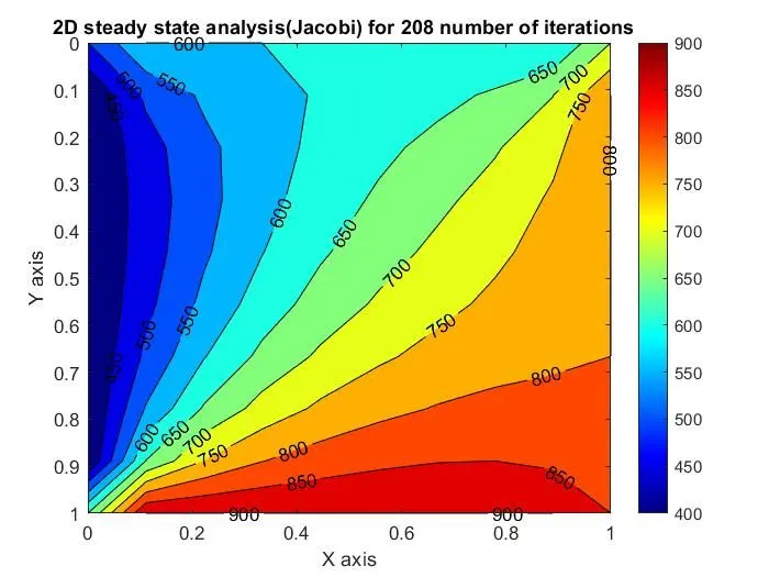
1. Jacobi
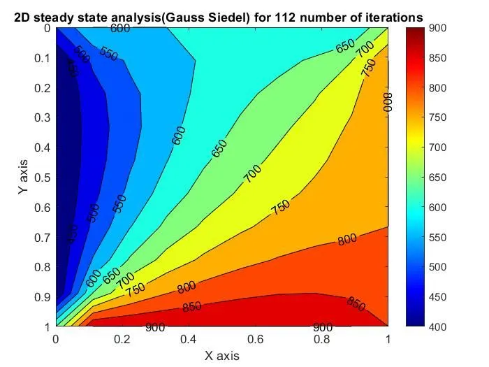
2. Gauss Siedel
3. Successive over relaxation
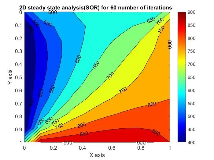
Explanation - The graphs generated for heat conduction are essentially same for all the three iterative methods; the only difference being in the iterations/ time taken to reach the solution which is visible at the top of each figure.
The flow of heat is always from region of higher temperature to that of a lower temperature.
The graph is complient with the priciple as various lines generated show the behaviour as described.
The Gauss Siedel(GS) method is an improvement on the Jacobi method. The Jacobi is slower as it uses the values from previous iteration, whereas, Gauss Siedel(GS) uses the updated value from the previous step.
The Successive Over Relaxation(SOR) method is an improvement on the GS method. The SOR iterations depend on the omega value given and that determines the rate of convergence.
For the solution obtained, omega = 1.3.
The rate of convergence is in the order of SOR>GS>Jacobi.
Program for unsteady state:
%Transient state

clear all
close all
clc

nx=10;
ny=10;
t=ones(nx,ny);

t(1,:)=600;
% method=0;
t(:,1)=400;
t(:,ny)=800;
t(nx,:)=900;
t(1,1)=500;
t(10,1)=650;
t(1,10)=700;
t(10,10)=850;
t(2:nx-1,2:ny-1)=300;
x=linspace(0,1,nx);
y=linspace(0,1,ny);
dx=1/(nx-1);
dy=1/(ny-1);
[xx yy] = meshgrid(x,y);
alpha=1.5;
dt=0.001;
k1= alpha*dt/dx^2;
k2= alpha*dt/dy^2;
error = 9e9;
tol=1e-4;
told1=t;
told2=t;
tp=t;
told3=t;
% t2=t
tinitial = t;
j_iter=1;
gs_iter=1;
w=0;
a1=1.5;
dt=0.001;
t_tot=1;
t_tot = t_tot/dt;
%nt = 30;
%k = a1*dt/(dx^2);

% CFL criteria for stability
CFL = a1*dt/(dx^2);


method=input('Enter method number 1. explicit 2. Impliclit Jacobi 3. Implicit Gauss Siedel 4. Implicit SOR');
% method=4;
nt=1400;
% Jacobi
if (method==1)


    for o=1:nt

        for i=2:nx-1

            for j=2:ny-1

                term1= (told1(i-1,j)+told1(i+1,j));
                term2= (told1(i,j-1)+told1(i,j+1));
                t(i,j)= told1(i,j)*(1-2*k1-2*k2)+k1*term1+k2*term2;
            end
        end
        error = max(max(abs(told1-t)));
        told1=t;
    end

    % Contour plot

    contourf(x,y,t,'showtext','on')
    colormap("jet")
    colorbar
    set(gca, 'YDIR', 'reverse')

    xlabel('X axis')
    ylabel('Y axis')
    title(sprintf('2D transient analysis by explicit scheme'))
    pause(0.03)
end

% Jacobi method - Implicit

if (method ==2)

    % Time step iteration
    for o=1:nt
        error=9e9;
        while error>tol
            for i=2:nx-1
                %Space step iteration
                for j=2:ny-1
                    term1=(1+(4*k1))^-1;
                    term2=k1*term1;
                    H = (told1(i-1,j)+told1(i+1,j));
                    V = (told1(i,j-1)+told1(i,j+1));
                    t(i,j)=(tp(i,j)*term1)+(H*term2)+(V*term2);
                end
            end
            a = abs ((t-told1));
            b = max (max(a));
            error = b;
            told1=t;
            j_iter = j_iter+1;
        end
        tp=told1;
    end
contourf(x,y,t,'showtext','on')
colormap(jet)
colorbar
set(gca,'YDIR','reverse')
xlabel('X axis')
ylabel('Y axis')
title (sprintf('2D transient analysis by implicit Jacobi method'))
pause(0.03)
end


% Gauss Seidel

if (method ==3)

    % Time step iteration
    for o=1:nt
        error=9e9;
        while error>tol
            %Space step iteration
            for i = 2:nx-1
                for j=2:ny-1
                    term1=(1+(4*k1))^-1;
                    term2=k1*term1;
                    H = (t(i-1,j)+told2(i+1,j));
                    V = (t(i,j-1)+told2(i,j+1));
                    t(i,j)=(tp(i,j)*term1)+(H*term2)+(V*term2);
                end
            end
            a = abs ((t-told2));
            b = max (max(a));
            error = b;
            told2=t;
            gs_iter = gs_iter+1;
        end
        tp=told2;
    end

    contourf(x,y,t,'showtext','on')
    colormap(jet)
    colorbar
    set(gca,'YDIR','reverse')
    xlabel('X axis')
    ylabel('Y axis')
    title (sprintf('2D transient analysis by implicit Gauss Siedel method'))
    pause(0.03)
end

% Successive Over Relaxation

if (method ==4)
    w = input('Enter the omega value for SOR');

sor_iter=1;
    % Time step iteration
    for o=1:nt
        error=9e9;
        while error>tol
            %Space step iteration
            for i = 2:nx-1
                for j=2:ny-1
                    term1=(1+(4*k1))^-1;
                    term2=k1*term1;
                    H = (t(i-1,j)+told3(i+1,j));
                    V = (t(i,j-1)+told3(i,j+1));
%                     t(i,j)=(1-w)*told3(i,j)+ w*tp(i,j)*term1;
                    t(i,j)=(1-w)*told3(i,j)+w*((tp(i,j)*term1)+((H)*term2)+((V)*term2));
                end
            end
            a = abs ((t-told3));
            b = max (max(a));
            error = b;
            told3=t;
            sor_iter = sor_iter+1;
        end
        tp=told3;
    end
    contourf(x,y,t,'showtext','on')
    colormap(jet)
    colorbar
    set(gca,'YDIR','reverse')
    xlabel('X axis')
    ylabel('Y axis')
    title (sprintf('2D transient analysis by implicit SOR method'))
    pause(0.03)

end
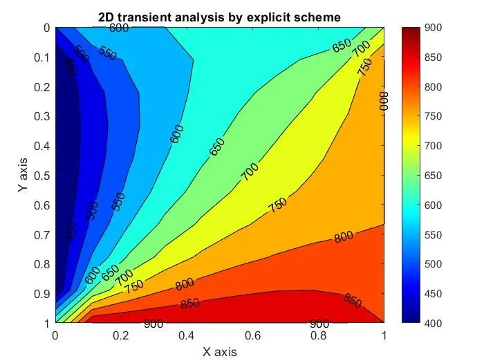
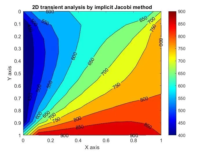
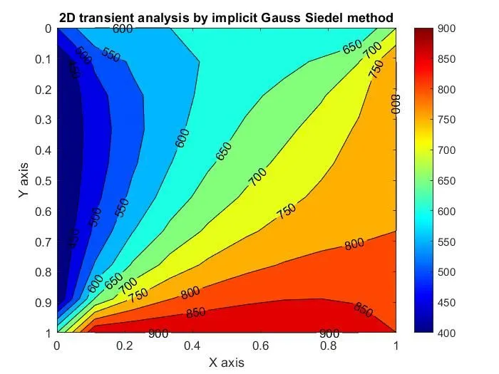
Solution graphs for unstady state:
1. Explicit scheme
2. Implicit scheme - jacobi
3. Implicit scheme - Gauss Siedel
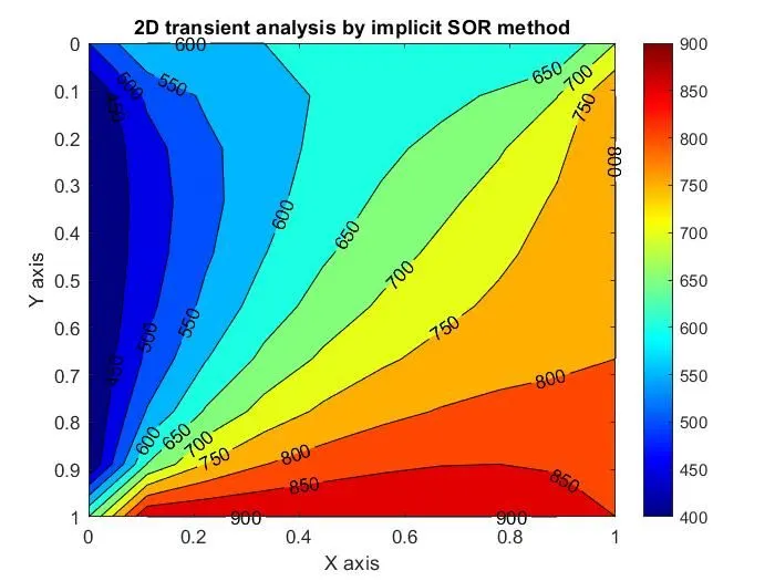
4. Implicit scheme - Succesive over Relaxation (Omega = 1.3)