Week 7 - Simulation of a 1D Super-sonic nozzle flow simulation using Macormack Method

Aim:-

• To simulate the isentropic flow through a quasi 1D subsonic-supersonic nozzle.
• To derive the conservation and non conservation forms of the governing equations and solve them using the MacCormack's technique.
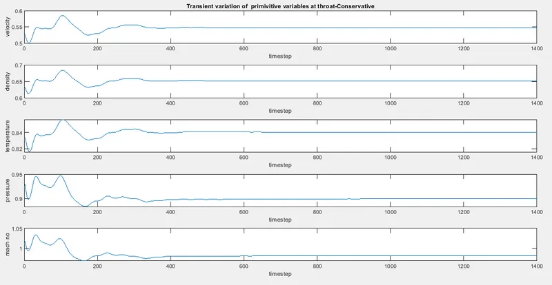
• To plot the distribution of primitive variables at throat for both the forms.
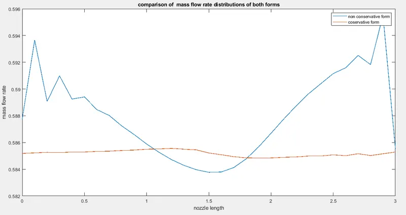
• To see the difference between the two forms of governing equations by comparing the solutions.

Theory:-

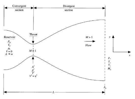
Schematic for subsonic-supersonic isentropic nozzle.

Inputs- CFD,applications J.D Anderson pg no.285

• The governing equations will be expressed in terms of PDE suitable for time marching solution of quasi 1D flow.
• Calculations of timesteps and boundary conditions .

Governing equations

Non conservative form

Continuity equation

`(partialrho')/(partialt')=-rho'.(partialV')/(partialx')-rho'.V'.(partial(lnA'))/(partialx')-V'.(drho')/(dx')`

Momentum equation

`(partialV')/(partialt')=-V.(partialV')/(partialx')-1/gamma.((partialT')/(partialx')+(T')/(rho').(partialrho')/(partialx'))`

Energy equation

`(partialT')/(partialt')=-V'.(partialT')/(partialx')-(gamma-1).T'((partialV')/(partialx')+V'.(partial(lnA'))/(partialx'))`

Conservative form

continuity equation

`(partial(rho'.A'))/(partialt')+(partial(rho'.A'.V'))/(partialx)=0`

Momentum equation

`(partial(rho'.A'.V'))/(partialt')+(partial(rho'.A'.V^2+(1/gamma)rho'A'))/(partialx')=(1/gamma)rho'((partialA')/(partialx'))`

Energy equation

`(partial(rho'.((e')/(gamma-1)+gamma/2.V^2).A'))/(partialt')+(partial(rho'.((e')/(gamma-1)+gamma/2.V^2).V'.A'+rho',A'.V'))/(partialx')=0`

The above equation can be written as

`(partialU1)/(partialt')=(partialF1)/(partialx')`

`(partialU2)/(partialt')=(partialF2)/(partialx')+J2`

`(partialU3)/(partialt')=(partialF3)/(partialx')`

`F_1=U_2`

`F_2=U_2^2/U_1+(gamma-1)/gamma.(U_3-gamma/2.U_2^2/U_1)`

`F_3=(gamma.U_2.U_3)/U_1-(gamma.(gamma-1))/2.U_2^3/U_1^2`

`J_2=1/gamma.rho'.T'.(partialA')/(partialx')`

Meshing

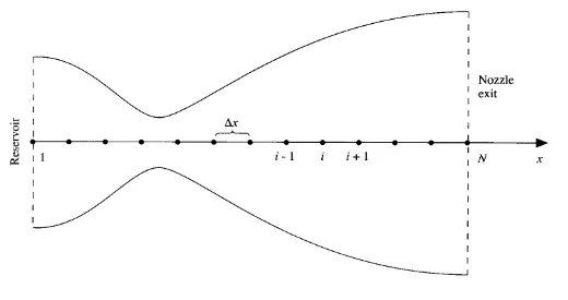
Discretization

Predictors step

`(partialf)/(partialt_p)=`Forward difference of the space terms.(derivatives wrt x)

Solution update

`f^*=f_i+(partialf)/(partialt_p).trianglet`

Corrector step

`(partialf^*)/(partialt_c)=`Backward diffrence of the space terms (derivatives wrt x)

`(partialf)/(partialt_(avg))=0.5.((partialf)/(partialt_p)+(partialf)/(partialt_c))`

Final solution update

`f^2=f_i+(partialf)/(partialt_(avg)).trianglet`

Boundary conditions

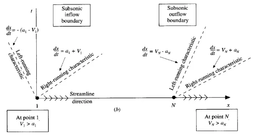
Some important formulae

Nozzle area,`A=1+2.2.(x-1.5)^2where0lexle3`

Pressure,`p=rho.T`

Mach no=`V/sqrtT`

Mass flow rate=`rho.A.V`

Matlab Code

Main code

clear all
close all
clc
% inputs
L=3;
n=31;
x=linspace(0,L,n);
dx=x(2)-x(1);
a=1+2.2*(x-1.5).^2; %area




tic
[t,rho,p,v,M,m,rho_throat,p_throat,t_throat,M_throat,v_throat]=non_conservative_form(n,x,dx);
time1=toc;
tic
[t_c,rho_c,p_c,v_c,M_c,m_c,rho_throat_c,p_throat_c,v_throat_c,t_throat_c,M_throat_c]=conservative_form(n,x,dx);
time2=toc;

figure(1)
subplot(5,1,1)
plot(x,t)
xlabel('nozzle length')
ylabel('Temperature')
title('Non-Cons form- Distribution of variables along the nozzle length')
subplot(5,1,2)
plot(x,rho)
xlabel('nozzle length')
ylabel('density')
subplot(5,1,3)
plot(x,p)
xlabel('nozzle length')
ylabel('pressure')
subplot(5,1,4)
plot(x,M)
xlabel('Nozzle length')
ylabel('mach no')
subplot(5,1,5)
plot(x,v)
xlabel('Nozzle length')
ylabel('velocity')

figure(3)
legend('1st timestep','50th timestep','100th timestep','200th timestep','1400th timestep')
title('non coservative form - variation of mass flow rate distribution at different time steps')
xlabel('nozzle length')
ylabel('mass flow rate')

figure(5)
subplot(5,1,1)
plot(v_throat_c)
xlabel('timestep')
ylabel('velocity')
title('Transient variation of  primivitive variables at throat-Conservative') 
subplot(5,1,2)
plot(rho_throat_c)
xlabel('timestep')
ylabel('density')
subplot(5,1,3)
plot(t_throat_c)
xlabel('timestep')
ylabel('temperature')
subplot(5,1,4)
plot(p_throat_c)
xlabel('timestep')
ylabel('pressure')
subplot(5,1,5)
plot(M_throat_c)
xlabel('timestep')
ylabel('mach no')

figure(7)
subplot(5,1,1)
plot(x,v_c)
xlabel('nozzle length')
ylabel('velocity')
title('steady state primivitive variable profiles- conservative') 
subplot(5,1,2)
plot(x,rho_c)
xlabel('nozzle length')
ylabel('density')
subplot(5,1,3)
plot(x,t_c)
xlabel('nozzle length')
ylabel('temperature')
subplot(5,1,4)
plot(x,p_c)
xlabel('nozzle length')
ylabel('pressure')
subplot(5,1,5)
plot(x,M_c)
xlabel('nozzle length')
ylabel('mach no')




figure(4)
subplot(5,1,1)
plot(v_throat)
xlabel('timestep')
ylabel('velocity')
title('Transient variation of  primivitive variables at throat-Non conservative form') 
subplot(5,1,2)
plot(rho_throat)
xlabel('timestep')
ylabel('density')
subplot(5,1,3)
plot(t_throat)
xlabel('timestep')
ylabel('temperature')
subplot(5,1,4)
plot(p_throat)
xlabel('timestep')
ylabel('pressure')
subplot(5,1,5)
plot(M_throat)
xlabel('timestep')
ylabel('mach no')

 figure(6)
xlabel('nozzle length')
ylabel('mass flow rate')
legend('50dt','100dt','250dt','500dt','700dt','1400dt')
title('Conservative variation of mass flow rate at different timesteps')


figure(8)
plot(x,m,'linewidth',1)
hold on
plot(x,m_c,'linewidth',1)
hold on
legend('non conservative form','coservative form')
xlabel('nozzle length')
ylabel('mass flow rate')
title('comparison of  mass flow rate distributions of both forms')

Function code

Non Conservative form

function[t,rho,p,v,M,m,rho_throat,v_throat,p_throat,t_throat,M_throat]=non_conservative_form(n,x,dx)
%  calculate initial profiles
rho=1-0.3146*x;
t=1-0.2314*x;
v=(0.1+1.09*x).*(t).^0.5;
gamma=1.4;
a=1+2.2*(x-1.5).^2; % area
% time steps
nt=1400;

th=16;
cfl =0.5; % CFL number
dt=min(dx.*(cfl)./(sqrt(t)+v));
%outer time step
for k=1:nt
    dt=min(dx.*(cfl)./(sqrt(t)+v));
    rho_old=rho;
    v_old=v;
    t_old=t;
    % predictor method
    
    for j=2:n-1
        dvdx=(v(j+1)-v(j))/dx;
       drhodx=(rho(j+1)-rho(j))/dx;
       dtdx=(t(j+1)-t(j))/dx;
       dlogadx=(log(a(j+1))-log(a(j)))/dx;
   
       % continuity equation
       drhodt_p(j)=-rho(j)*dvdx-rho(j)*v(j)*dlogadx-v(j)*drhodx;
       
       %momentum equation
       dvdt_p(j)=-v(j)*dvdx-(1/gamma)*(dtdx+(t(j)/rho(j))*drhodx);
       
       % energy  equation
       dtdt_p(j)=-v(j)*dtdx-(gamma-1)*t(j)*(dvdx+v(j)*dlogadx);
       
       % solution update 
     rho(j)=rho(j)+drhodt_p(j)*dt;
     v(j)= v(j)+ dvdt_p(j)*dt;
     t(j)=t(j)+dtdt_p(j)*dt;
    end
    % corrector method  
    for j=2:n-1
        dvdx=(v(j)-v(j-1))/dx;
       drhodx=(rho(j)-rho(j-1))/dx;
       dtdx=(t(j)-t(j-1))/dx;
       dlogadx=(log(a(j))-log(a(j-1)))/dx;
   
       % continuity equation
       drhodt_c(j)=-rho(j)*dvdx-rho(j)*v(j)*dlogadx-v(j)*drhodx;
       
       %momentum equation
       dvdt_c(j)=-v(j)*dvdx-(1/gamma)*(dtdx+(t(j)/rho(j))*drhodx);
       
       % energy  equation
       dtdt_c(j)=-v(j)*dtdx-(gamma-1)*t(j)*(dvdx+v(j)*dlogadx);
       
      
    end
     % average time derivative
    drhodt=0.5*(drhodt_p+drhodt_c);
    dvdt=0.5*(dvdt_p+dvdt_c);
    dtdt=0.5*(dtdt_p+dtdt_c);
    
    % final solution update
    for i=2:n-1
        rho(i)=rho_old(i)+drhodt(i)*dt;
        v(i)=v_old(i)+dvdt(i)*dt;
        t(i)=t_old(i)+dtdt(i)*dt;
    end
     % boundary conditions
    % inlet 
    v(1)=2*v(2) -v(3);
    % outlet
    v(n)=2*v(n-1)-v(n-2);
    rho(n)=2*rho(n-1)-rho(n-2);
    t(n)=2*t(n-1)-t(n-2);
    % pressure
    p=rho.*t;
    % mach number
    M=v./sqrt(t);
    %mass flow rate
    m=rho.*a.*v;
 
    if k==1
        figure(3)
        plot(x,m)
        hold on
    end
     if k==100
         figure(3)
        plot(x,m)
        hold on
    end
     if k==250
         figure(3)
        plot(x,m)
        hold on
    end
     if k==500
         figure(3)
        plot(x,m)
        hold on 
    end
     if k==700
         figure(3)
        plot(x,m)
        hold on 
    end
     if k==1400
         figure(3)
        plot(x,m)
        hold on
    end
    v_throat(k)=v(th);
    rho_throat(k)=rho(th);
    t_throat(k)=t(th);
    p_throat(k)=p(th);
    M_throat(k)=M(th);

end
figure(3)
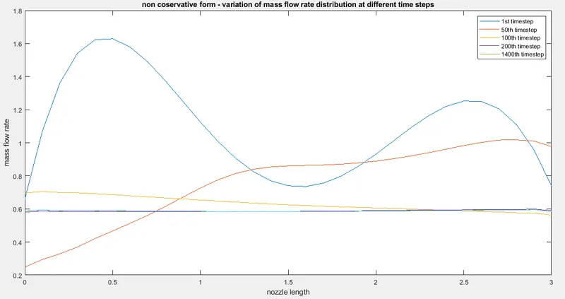
legend('1st timestep','50th timestep','100th timestep','200th timestep','1400th timestep')
title('non coservative form - variation of mass flow rate distribution at different time steps')
xlabel('nozzle length')
ylabel('mass flow rate')


        

Function code

Conservative Form

function[t_c,rho_c,p_c,v_c,M_c,m_c,rho_throat_c,v_throat_c,p_throat_c,t_throat_c,M_throat_c]=conservative_form(n,x,dx)

gamma=1.4;
th=16;

for i=1:n
   if x(i)<=0.5
       rho_c(i)=1;
       t_c(i)=1;
   end
    if x(i)>0.5 && x(i)<=1.5
        rho_c(i)=1-0.366*(x(i)-0.5);
        t_c(i)=1-0.167*(x(i)-0.5);
    end
     if x(i)>1.5
        rho_c(i)=0.634-0.3879*(x(i)-1.5);
        t_c(i)=0.833-0.3507*(x(i)-1.5);
    end
end
% timesteps
nt=1400;



% area
a=1+2.2*(x-1.5).^2;
v_c=0.59./(rho_c.*a);
U1=rho_c.*a;
U2=rho_c.*a.*v_c;
U3=U1.*(t_c/(gamma-1)+(gamma/2)*v_c.^2);
cfl=0.5; % CFL number


F1=U2;
F2=U2.^2./U1+(gamma-1)/(gamma)*(U3-(gamma/2)*U2.^2./U1);
F3=gamma*U2.*U3./U1-0.5*gamma*(gamma-1)*(U2.^3./U1.^2);



 
for k=1:nt
    %copy of values U1,U2,U3
   U1_old=U1;
   U2_old=U2;
   U3_old=U3;
   dt=min(dx.*(cfl)./(sqrt(t_c)+v_c));   
   
F1=U2;
F2=U2.^2./U1+(gamma-1)/(gamma)*(U3-(gamma/2)*U2.^2./U1);
F3=gamma*U2.*U3./U1-0.5*gamma*(gamma-1)*(U2.^3./U1.^2);

   
   
    % predictor method
   
    for j=2:n-1
      
       % continuity equation
       dU1dt_p(j)=-(F1(j+1)-F1(j))/dx;
       
        J2=(1/gamma)*rho_c(j)*t_c(j)*((a(j+1)-a(j))/dx);
       %momentum equation
      dU2dt_p(j)=-(F2(j+1)-F2(j))/dx+J2;
       
       % energy  equation
     dU3dt_p(j)=-(F3(j+1)-F3(j))/dx;
       
       % solution update
     U1(j)=U1(j)+dU1dt_p(j)*dt;
     U2(j)= U2(j)+ dU2dt_p(j)*dt;
     U3(j)=U3(j)+dU3dt_p(j)*dt;
    end
   
    %predictor update
    rho_c=U1./a;
    t_c=(gamma-1)*(U3./U1-(gamma/2)*(U2./U1).^2);
    F1=U2;
    F2=U2.^2./U1+(gamma-1)/(gamma)*(U3-(gamma/2)*U2.^2./U1);
    F3=gamma*U2.*U3./U1-0.5*gamma*(gamma-1)*(U2.^3./U1.^2);


   
    % corrector method  
    for j=2:n-1
        % continuity equation
       dU1dt_c(j)=-(F1(j)-F1(j-1))/dx;
       
        J2=(1/gamma)*rho_c(j)*t_c(j)*((a(j)-a(j-1))/dx);
       %momentum equation
      dU2dt_c(j)=-(F2(j)-F2(j-1))/dx +J2;
       
       % energy  equation
     dU3dt_c(j)=-(F3(j)-F3(j-1))/dx;
       
       
     
    end
     % average time derivative
    dU1dt=0.5*(dU1dt_p+dU1dt_c);
    dU2dt=0.5*(dU2dt_p+dU2dt_c);
    dU3dt=0.5*(dU3dt_p+dU3dt_c);
   
    %final solution update
    for i=2:n-1
        U1(i)=U1_old(i)+dU1dt(i)*dt;
        U2(i)=U2_old(i)+dU2dt(i)*dt;
        U3(i)=U3_old(i)+dU3dt(i)*dt;
    end
   
   
   
     % boundary conditions
    % inlet
  U1(1)=rho_c(1)*a(1);
  U2(1)=2*U2(2)-U2(3);
  U3(1)=U1(1)*(t_c(1)/(gamma-1)+0.5*gamma*v_c(1)^2);
    % outlet
    U1(n)=2*U1(n-1)-U1(n-2);
    U2(n)=2*U2(n-1)-U2(n-2);
    U3(n)=2*U3(n-1)-U3(n-2);
     %final update
    rho_c=U1./a;
    t_c=(gamma-1)*(U3./U1-(gamma/2)*(U2./U1).^2);
    v_c=U2./U1;
   
   % pressure
    p_c=rho_c.*t_c;
    % mach number
    M_c=v_c./sqrt(t_c);
    %mass flow rate
    m_c=rho_c.*a.*v_c;
   
   
   
    if k==50
        figure(6)
        plot(x,m_c)
        hold on
    end
     
     if k==100
          figure(6)
          plot(x,m_c)
        hold on
     end
     
     if k==250
          figure(6)
         plot(x,m_c)
        hold on
    end
     if k==500
          figure(6)
         plot(x,m_c)
        hold on
    end
     if k==700
          figure(6)
         plot(x,m_c)
        hold on
    end
     if k==1400
          figure(6)
         plot(x,m_c)
         
         xlabel('nozzle length')
        ylabel('mass flow rate')
           legend('50dt','100dt','250dt','500dt','700dt','1400dt')
title('Conservative variation of mass flow rate at different timesteps')

        hold off
       
       
     end
   
     
    v_throat_c(k)=v_c(th);
    rho_throat_c(k)=rho_c(th);
    t_throat_c(k)=t_c(th);
    p_throat_c(k)=p_c(th);
    M_throat_c(k)=M_c(th);
   
end
    
    

Explanation:-

• Initially the grid size(n),x and x values are assigned.
• Then the function code for non-conservation form is executed.Under the function, initial profiles (rho,T,V), area of nozzle,timestep values are assigned.
• Loop for outer time step is initiated under which the copy of variables (rho,T,V) is created and the Macormacks method is carried out.
• Predictor method followed by solution update is done .Corrector method followed by final solution update is also done.
• The boundary conditions at the inlet and outlet are given.Then pressure ,mach no and mass flow rate are calculated.
• Then the values of primitive variables at the throat are assigned to variables with size k so that for each timestep,the values at throat are calculated.
• Then the mass flow rates at different time steps are plotted.
• The above process is repeated for 1400 time stepsand the function returns the final values of primitive variables to the main program.
• Then the function with conservation form is executed.The same process as followed in non conservation form is repeated except that flux vectors (F1,F2,F3) an the solutions vectors (U1,U2,U3) are used in this form.
• In Maccormack's method, the flux vectors and the solutions vectors are used and then primitive variables are updated.
• The above process s repeated for 1400-time steps and the function returns the final values of primitive variables to the main program.
• The simulation time for the conservation form and non- conservation form are stored in variables time,time2 respectively.
• Then finally the respective plots are obtained using figure and subplot commands.

Output Plots:-

Non-conservative plots

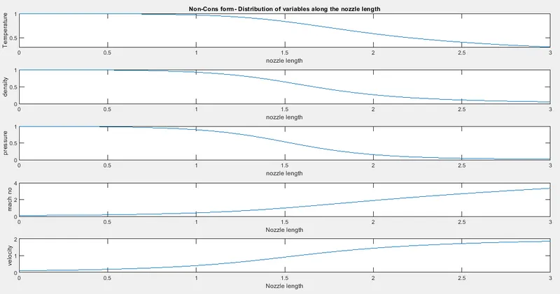
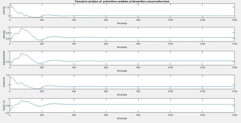
Conservative form

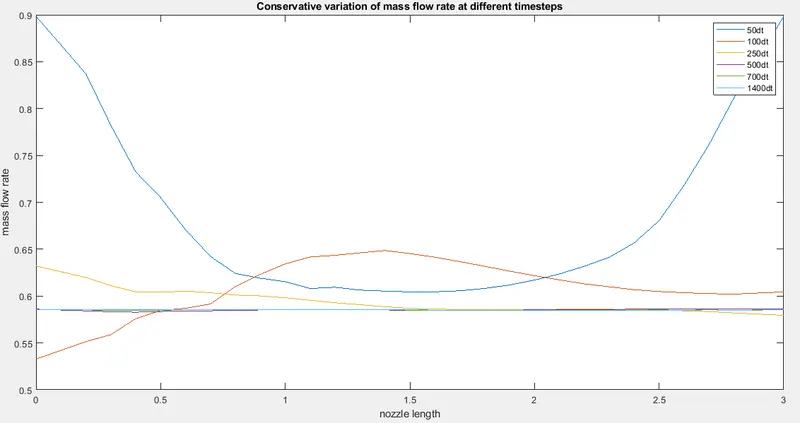
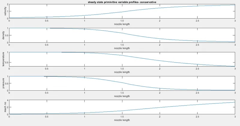
Comparision of both the forms Non-conservative and Conservative form

Conclusion

• Using MATLAB, the isentropic floe through a quasi 1D subsonic-supersonic nozzle is simulated.
• The conservation and non-conservation forms of the governing equation were solved using Macormack technique.
• Distribution of primitive variables, mass flow rate through nozzle and time-wise variations of primitive variables at throat were plotted for both of the forms.
• Both comparision ofconservation an non-conservation forms are plotted.