Week 5.1 - Mid term project - Solving the steady and unsteady 2D heat conduction problem
Solving steady and unsteady 2D heat conduction problem
Aim:- To write codes to solve 2D heat conduction equation by using iterative techniques by implementing the following techniques
1) Jacobi
2) Gauss Seidal
3) Sucessive Over Relaxation
Introduction:-
Considering 3 Dimensional heat conduction equation
`(∂T)/(∂t)+alpha((∂^2T)/(∂x^2)+(∂^2T)/(∂y^2)+(∂^2T)/(∂z^2))`=0
above equation has 2 terms ie term1 is time domain , term2 is spatial deravative and `alpha`is thermal diffusivity factor Solution is assumed as thin plate Z direction is neglected
`∂T/∂t+alpha((∂^2T)/(∂x^2)+(∂^2T)/(∂y^2))=0`
Above equation can be solved using two methods
Explicit method
Implicit method
Assumptions
1) Assume domain is a square unit
2) Assume nx=ny=10(steady),nx=ny=41(unsteady)
3) Boundary Conditions
left=400k
Top=600k
Right=800k
Bottom=900k
4) tolerance =1e-4
5) start error-9e9
6) Thermal diffusivity (Alpha)=1.88e-5 m^2/s
7)Domain length =1m
8) CFL(for stability)= alpha *`(dt/dx^2)`
Solving steady state equation `(∂^2T)/(∂x^2)+(∂^2T)/(∂y^2)=0`
her discretizing the equation by appliying central differencing scheme
`T(i,j)={(Told(i-1,j)+Told(i+1,j))/dx^2)+((Told(i,j-1)+Told(i,j+1))/dy^2)}`
`k=2*((dx^2+dy^2)/(dx^2*dy^2))`
Code for solving three iterative solvers
 % solving steady state equation by employing
    %different solvers like jacobi, gauss seidal, sucessive over relaxation

    clear all
    close all
    clc
    % defining the inputs
    L=1;
    nx=10;
    ny=nx;
    x=linspace(0,1,nx);
    y=linspace(0,1,ny);
    dx=x(2)-x(1);
    dy=y(2)-y(1);
    [xx,yy]=meshgrid(x,y);
    % defining the boundary conditions
    T=ones(nx,ny);
    T(1,:)=900;
    T(end,:)=600;
    T(:,1)=400;
    T(:,end)=800;
    Told=T;
    % error_tol,start_error
    error_tol=1e-4;
    start_error=9e9;
    k=2*((dx^2+dy^2)/(dx^2*dy^2));
    % defining the solver
    iterative_solver=input('enter the desired number with respect to solver:');


      if   iterative_solver==1
              tic;
              T_jacobi=jacobi_iter(start_error,error_tol,xx,yy,nx,ny,dx,dy,T,k,Told);
        time_jacobi_in_sec=toc;

      elseif  iterative_solver ==2
        tic;
         T_gauss=gauss_iter(start_error,error_tol,xx,yy,nx,ny,dx,dy,k,T,Told);
            time_gauss_in_sec=toc;


              elseif iterative_solver==3
                tic;
                T_sor_iter=sor_iter(start_error,error_tol,x,y,nx,ny,dx,dy,k,T,Told);
                time_sor_in_sec=toc;
            end
Function code for jacobi:-
% function for jacobi method to solve steady state equation
function T =jacobi_iter(start_error,error_tol,xx,yy,nx,ny,dx,dy,T,k,Told)
jacobi_iter=1;
while(start_error>error_tol)
    for i=2:nx-1
     for   j=2:ny-1
        term1=(Told(i-1,j)+Told(i+1,j))/(k*(dx^2));
        term2=(Told(i,j+1)+Told(i,j-1))/(k*(dy^2));
        T(i,j)=term1+term2;
    end
    end
start_error=max(max(abs(Told-T)));
Told=T;
jacobi_iter=jacobi_iter+1;
figure(1)
[c,d]=contourf(xx,yy,T);
colormap(jet)
colorbar
title_text=sprintf('Jacobi iteration number=%d@steady state',jacobi_iter);
title(title_text)
xlabel('x-axis')
ylabel('y-axis')
clabel(c,d)
pause(0.03)
end
fprintf('no of iteration in jacobi=%d',jacobi_iter);
end
Function code for gauss iter:-
% function for gauss_seidal method to solve steady state equation
function T =gauss_iter(start_error,error_tol,xx,yy,nx,ny,dx,dy,k,T,Told)
GS_iter=1;

while(start_error>error_tol)
    for i=2:nx-1
     for   j=2:ny-1
         term1=(T(i-1,j)+Told(i+1,j))/dx^2;
         term2=(T(i,j-1)+Told(i,j+1))/dy^2;
        T(i,j)=(term1+term2)/k;
    end
    end
start_error=max(max(abs(Told-T)));
Told=T;
GS_iter=GS_iter+1;
figure(2)
[c,d]=contourf(xx,yy,T);
colormap(jet)
colorbar
title_text=sprintf('GS iteration number=%d@steady state',GS_iter);
title(title_text)
xlabel('x-axis')
ylabel('y-axis')
clabel(c,d)
pause(0.03)
end
fprintf('no of iteration in GS=%d',GS_iter);
end
Function code for Sucessive Over Relaxation:-
% function for SOR method to solve steady state equation
function T =sor_iter(start_error,error_tol,x,y,nx,ny,dx,dy,k,T,Told)
sor_iter=1;
omega=1.7;
while(start_error>error_tol)
    for i=2:nx-1
     for   j=2:ny-1
         T_gs=((((T(i-1,j)+Told(i+1,j))/dx^2))+(((T(i,j-1)+Told(i,j+1))/dy^2)))/k;

         T(i,j)=omega*(T_gs)+(1-omega)*(Told(i,j));
    end
    end
start_error=max(max(abs(Told-T)));
Told=T;
sor_iter=sor_iter+1;
figure(1)
[c,d]=contourf(x,y,T);
colormap(jet)
colorbar
title_text=sprintf('SOR iteration number=%d@steady state',sor_iter);
title(title_text)
xlabel('x-axis')
ylabel('y-axis')
clabel(c,d)
pause(0.03)
end
fprintf('no of iteration in SOR=%d',sor_iter);
end
Results:-
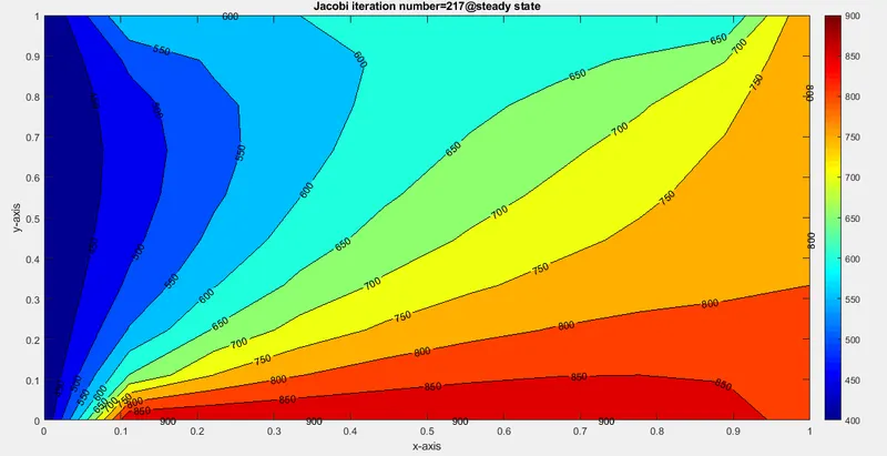
Enter the desired number with respect to solver:1
No of iteration =217
time taken to solve=54.214 secs
Gauss seidal:-
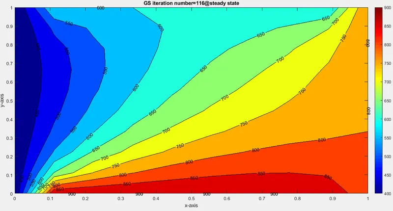
Enter the desired with respect to solver:2
no of iteration =116
time taken to solve=51
Sucessive Over Relaxation:-
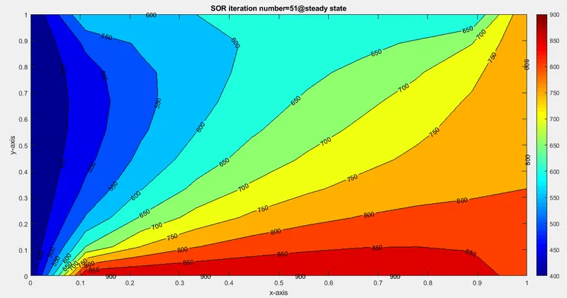
Enter the desired number with respect to solver :3
no of iteration =51
time taken to solve=14.708 secs
From all the above results it can be inferred that SOR method takes less iterations and less time to solve ,so SOR is best method among all.
Solving Transient state equation
Transient state steady conduction eqauation is solved in both ways explicitly and implicitly
`(∂T)/(∂t)+alpha((∂^2T)/(∂x^2)+(∂^2T)/(∂y^2))=0`
in this metod , each diferential equation approach contains only one unknown and can be solved explicitly for this one unknown using this method
Discretised equation
`T^(n+1)(i,j)=T^n+k1*(T^nold(i+1,j)-2*T^nold(i,j)+T^nold(i-1,j)+k2*(T^nold(i,j-1)-2*T^nold(i,j)+T^nold(i,j+1)` `k1=2*((alpha*dt)/dx^2),k2=2*((alpha*dt)/dy^2)`
code for 2D transient conduction equation solving explicitly:-
% solving 2D Transient heat conduction equation explicitly
clear all
close all
clc
% defining the inputs
nx=41;
ny=nx;
x=linspace(0,1,nx);
y=linspace(0,1,ny);
dx=x(2)-x(1);
dy=y(2)-y(1);
dt=0.01;
alpha=1.88e-5;% thermal diffusivity
[xx,yy]=meshgrid(x,y);
% defining boundary conditions
T=ones(nx,ny);
T(1,:)=900;
T(end,:)=600;
T(:,1)=400;
T(:,end)=800;
Told=T;
% roundingoff the corner values by taking the average values
T(1,1)=(400+900)/2;
T(1,ny)=(900+800)/2;
T(nx,1)=(400+600)/2;
T(nx,ny)=(600+800)/2;
% error_tol,start_error
error_tol=1e-4;
start_error=9e9;
k1=alpha*(dt/dx^2);
k2=alpha*(dt/dy^2);
% defining the solver
iterative_solver=1;
tic;
if iterative_solver==1
    T_jacobi=jacobi_iter_transient_expli(xx,yy,nx,ny,T,k1,k2,Told);
end
time_jacobi_in_sec=toc;
function code for explicit:-
% function for jacobi method to solve the transient state equation
% (explicit)
function T=jacobi_iter_transient_expli(xx,yy,nx,ny,T,k1,k2,Told)
jacobi_iter=1;
for k=1:120000
    for i=2:nx-1
        for j=2:ny-1
            term1=Told(i,j);
            term2=k1*(Told(i+1,j)-2*Told(i,j)+Told(i-1,j));
            term3=k2*(Told(i,j+1)-2*Told(i,j)+Told(i,j-1));
            T(i,j)=term1+term2+term3;
        end
    end
    start_error=max(max(abs(Told-T)));
    Told=T;
    jacobi_iter=jacobi_iter+1;
end
figure(1)
[c,d]=contourf(xx,yy,T);
colormap(jet)
colorbar
title_text=sprintf('Jacobi iteration number =%d@transient state explicitly',jacobi_iter');
title(title_text)
xlabel('x-axis')
ylabel('y-axis')
clabel(c,d)
pause(0.03)
fprintf('no of iteration in jacobi=%d\n',jacobi_iter);
end
Results:-
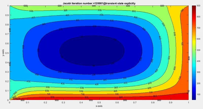
no of iteration =120001
time=5.28
Solving above equation implicitly
Implicit approach is used in numerical analysis for obtaining numerical approximations to the solution of time dependent ordinary or partial differential equations as in required in computer simulations of a physical process.
Here in this equation time deravative terms are calculated using the first order differential equation and whereas the term 2 has second order deravative terms and elliptical in nature so information need to be taken from all the points equally .so therefore a central differencing scheme is applied for the discretising the term2
The final discretised equation for 2D heat conduction equation for the implicit form is as follows:-
`T^(n+1)(i,j)=T^n+(k1*(T^nold(i+1,j)-2*T^nold(i,j)+T^nold(i-1,j))^(n+1)+(k2*[T^nold(i,j-1)-2*T^nold(i,j)+T^nold(i,j+1)]^(n+1)` k1,k2 as mentione above in explicit
equations for jacobi method are
term1 =(1+(2*k1)+(2*k2)^(-1);
term2=k1*term1;
term3=k2*term1;
H=(Told(i-1,j)+Told(i+1,j));
v=(Told(i,j-1)+Told(i,j+1));
T(i,j)=(Tprev(i,j)*term1)+term2*H+term3*v
the gauss seidal method is similar to the jacobi method but only difference is for the iteration vlue of T at a particular node is calculated .
once the value of T is found out iteratively whose error is ls than the tolerance value of T is calculated at the time time step n+2.
equations for gauss seidal are
term1 =(1+(2*k1)+(2*k2)^(-1);
term2=k1*term1;
term3=k2*term1;
H=(Told(i-1,j)+Told(i+1,j));
v=(Told(i,j-1)+Told(i,j+1));
T(i,j)=(Tprev(i,j)*term1)+term2*H+term3*v
SOR:
This method can be applied either by using jacobi or gauss seidal but the only difference is consideration of factor called omega(scaling factor) which in turn makes the process sooner ,iteration required to solve gets minimised
omega =2/(1+sin(pi*dx))
Equations for SOR :
term1=(1+(2*k1)+(2*k2))^-1;
term2=k1*term1;
term3=k2*term1;
h=(T(1-i,j)+Told(i+i,j));
v=(T(i,j-1)+Told(i,j+1));
T(i,j)=omega*(Tprev(i,j)*term1+term2*H+term3*v)+(1-omega)*Tprev(i,j)
code for 2D transient heat conduction equation solving implicitly
% solving 2D transient heat conuction equation implicitly
clear all
close all
clc
% defining the inputs
nx=41;
ny=nx;
L=1;
x=linspace(0,1,nx);
y=linspace(0,1,ny);
dx=x(2)-x(1);
dy=y(2)-y(1);
dt=0.01;
alpha=1.8-3;%thermal diffusivity
[xx,yy]=meshgrid(x,y);
%defining boundary conditions
T=298*ones(nx,ny);
T(1,:)=900;
T(end,:)=600;
T(:,1)=400;
T(:,end)=800;
% rounding off the corner value by taking the average value
T(1,1)=(400+900)/2;
T(1,ny)=(900+800)/2;
T(nx,1)=(400+600)/2;
T(nx,ny)=(600+800)/2;

Told=T;
Tprev=Told;
%error_tol,start_error
error_tol=1e-4;
start_error=9e9;
k1=alpha*(dt/dx^2);
k2=alpha*(dt/dy^2);
omega=2/(1+sin(pi*dx));
CFL=alpha*(dt/dx^2);
% defining three solvers
iterative_solver=input('input the appropriate number to select the required method:');
if iterative_solver==1
    tic;

       T_jacobi=jacobi_iter_trans_impli(error_tol,xx,yy,nx,ny,T,k1,k2,Told);
elseif iterative_solver==2
    tic;

    T_gs=gs_iter_trans_impli(error_tol,xx,yy,nx,ny,T,k1,k2,Told);
elseif iterative_solver==3
    tic;

    T_sor=sor_iter_trans_impli(error_tol,xx,yy,nx,ny,T,k1,k2,Told,omega);
end
function code for jacobi:-
%function for jacobi method transient state equation
function T=jacobi_iter_trans_impli(error_tol,xx,yy,nx,ny,T,k1,k2,Told)
jacobi_iter=1;
for k=1:120000 % time loop
    start_error=9e9;
    while(start_error > error_tol)% convergence loop
        for i=2:nx-1 % nodal loop
            for j=2:ny-1
                term1=(1+(2*k1)+2*k2)^-1;
                term2=k1*term1;
                term3=k2*term1;
                H=(T(i-1,j)+T(i+1,j));
                v=(T(i,j-1)+T(i,j+1));
                T(i,j)=(T(i,j)*term1)+H*term2+v*term3;

            end
        end
        start_error=max(max(abs(Told-T)));
        Told=T;
        jacobi_iter=jacobi_iter+1;
    end
    Tprev=T;
end
time_jacobi=toc;
contourf(xx,yy,T)
colormap(jet)
colorbar
xlabel('x-axis')
ylabel('y-axis')
colorbar
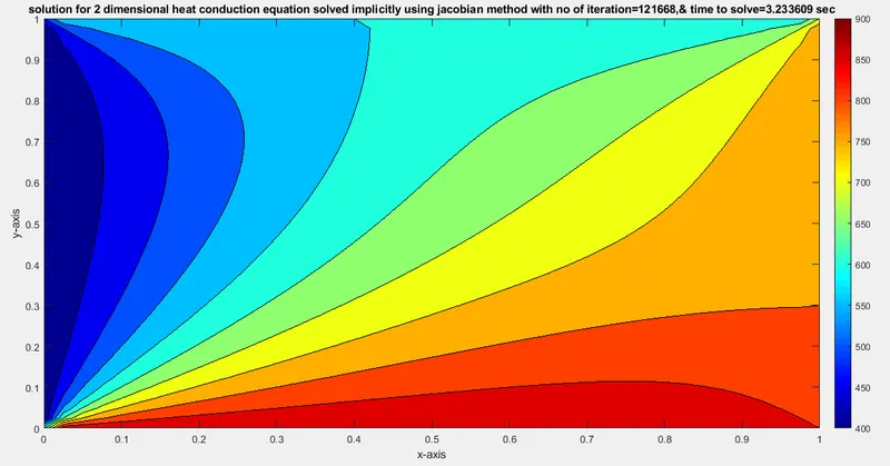
title_text=sprintf('solution for 2 dimensional heat conduction equation solved implicitly using jacobian method with no of iteration=%d,& time to solve=%f sec',jacobi_iter,time_jacobi');
title(title_text)
fprintf('no of iteration in jacobi =%d and time in sec=%f',jacobi_iter,time_jacobi);
pause(0.03)
end
function code for gauss seidal:
%function for GS method to transient state equation
function T=gs_iter_trans_impli(error_tol,xx,yy,nx,ny,T,k1,k2,Told)
gs_iter=1;
for k=1:120000 % time loop
    start_error=9e9;
    while(start_error > error_tol)% convergence loop
        for i=2:nx-1 % nodal loop
            for j=2:ny-1
                term1=(1+(2*k1)+(2*k2))^-1;
                term2=k1*term1;
                term3=k2*term1;
                H=(T(i-1,j)+T(i+1,j));
                V=(T(i,j-1)+T(i,j+1));
                T(i,j)=T(i,j)*term1+term2*H+term3*V;
            end
        end
        start_error=max(max(abs(Told-T)));
        Told=T;
        gs_iter=gs_iter+1;
    end
    Tprev=T;
end
time_gauss=toc;
contourf(xx,yy,T)
colormap(jet)
colorbar
xlabel('x-axis')
ylabel('y-axis')
colorbar
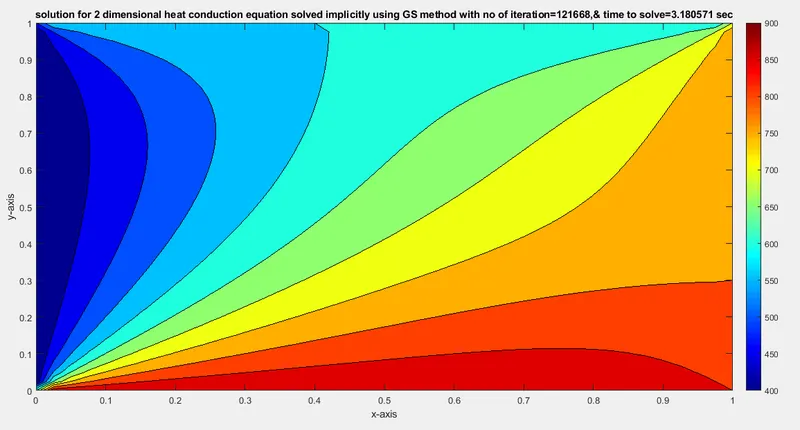
title_text=sprintf('solution for 2 dimensional heat conduction equation solved implicitly using GS method with no of iteration=%d,& time to solve=%f sec',gs_iter,time_gauss');
title(title_text)
fprintf('no of iteration in gauss iter =%d an time in sec=%f',gs_iter,time_gauss);
pause(0.03)
end
function code for SOR:
%function for sor method to transient state equation
function T=sor_iter_trans_impli(error_tol,xx,yy,nx,ny,T,k1,k2,Told,omega)
sor_iter=1;
for k=1:120000 % time loop
    start_error=9e9;
    while(start_error > error_tol)% convergence loop
        for i=2:nx-1 % nodal loop
            for j=2:ny-1
                term1=(1+(2*k1)+(2*k2))^-1;
                term2=k1*term1;
                term3=k2*term1;
                H=(T(i-1,j)+T(i+1,j));
                V=(T(i,j-1)+T(i,j+1));
                T(i,j)=omega*(T(i,j)*term1+term2*H+term3*V)+(1-omega)*T(i,j);
            end
        end
        start_error=max(max(abs(Told-T)));
        Told=T;
        sor_iter=sor_iter+1;
    end
    Tprev=T;
end
time_sor=toc;
contourf(xx,yy,T)
colormap(jet)
colorbar
xlabel('x-axis')
ylabel('y-axis')
colorbar
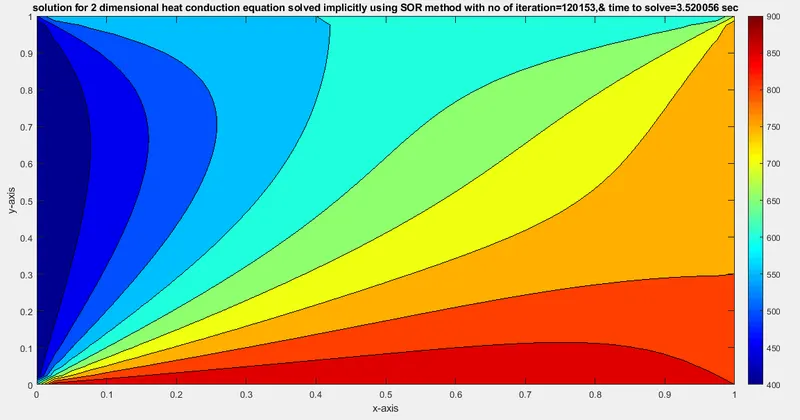
title_text=sprintf('solution for 2 dimensional heat conduction equation solved implicitly using SOR method with no of iteration=%d,& time to solve=%f sec',sor_iter,time_sor');
title(title_text)
fprintf('no of iteration in sor iter =%d an time in sec=%f',sor_iter,time_sor);
pause(0.03)
end
Results:
Jacobi
Gauss seidal:
SOR:
Conclusion:
1) In steady state equations SOR takes less time to solve compare to other two methods.
So it better to use SOR to yield faster results.
2) For stable solutions it is better to use steady state equations rather than transient state equation .