Week 7 - Simulation of a 1D Super-sonic nozzle flow simulation using Macormack Method
AIM:
The objective of the report is to do simulation of 1D super-sonic nozzle flow using the Macormack method and validate the results.
PROBLEM STATEMENT -
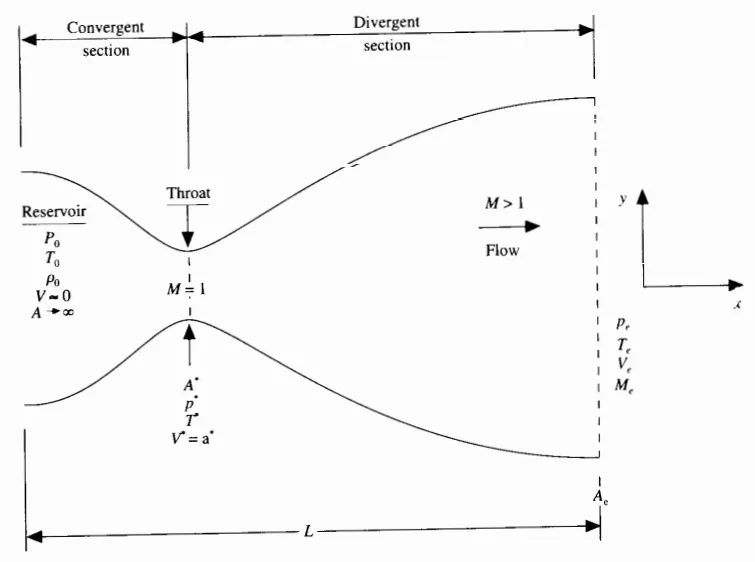
Given, a nozzle of length L, where the nozzle inlet is connected to a reservoir. The nozzle is designed in such a way that, in converging section, the Mach number is < 1 and in diverging section, the Mach number is > 1. At throat of the nozzle, the Mach number = 1.
Here, 1D flow field is considered which indicates that flow variables are changed in only x-direction. Due to pressure difference, the fluid flows through the nozzle. The working fluid considered in this analysis is air, that can be treated as ideal gas.
GOVERNING EQUATIONS -
In fluid dynamics, any problem can be represented by using 3 governing equations namely - continuity equation, momentum conservation equation and energy conservation equation.
FORMS OF PDE -
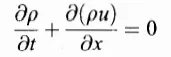
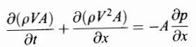
1) Conservative form - In conservative form, the control volume is assumed as stationary.
Continuity :
Momentum :
Energy :
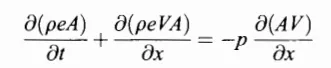 , where e - internal energy, (e=cvT)
2) Non - Conservative form - In non-conservative form, the control volume is moving.
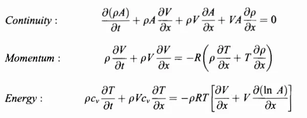
The above equations are expressed in terms of their dimensional forms. In this report, we are expressing the above equations in their non-dimensional form. The field variables are expressed in terms of reservoir values as given below
 , T' is non dimensional form of temperature.
 , ρ' is non dimensional form of density.
 , x' is non dimensional form of length.
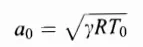 , a0 is speed of sound in reservoir
 , v' is non dimensional form of speed.
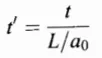 , t' is non dimensional form of time.
 , A' is non dimensional form of area, expressed in terms of throat area.
MACCORMACK'S METHOD -
In CFD, MacCormack method is widely used discretization scheme for the numerical solution of hyperbolic partial differential equations.
- It is a explicit finite difference method.
- It is a second order accurate in both space and time.
In this report, the numerical solution is obtained by using MacCormack method.
Let, ϕ is the flow field variable and the numerical solution s obtained by the following equation -
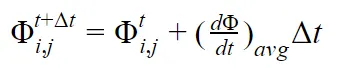
where, 
In predictor loop, forward difference method is used, at 't' time step.
In corrector loop, backward difference method is used, at 't+dt' time step.
PROCEDURE:
In this report, the governing equations are expressed in two forms as stated above and the results are validated.
1) Non - Conservative form -
The governing equations are expressed in terms of non dimensional terms



Time step -
The time step dt is calculate by using the following equation
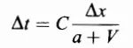 , where c - courant number, a - speed of sound in the medium, v - velocity of fluid.
The time sep dt is calculated for courant number C = 0.5. Each grid point has a different value of dt, so for stable solution minimum time step is considered.

Initial conditions -
The initial conditions are chosen in such a manner that it replicates the flow field. So, as the flow expands through the nozzle, the pressure and temperature decreases and velocity increases and these are represented in the below equations

NOZZEL SHAPE -

Boundary conditions -
In order to solve the governing equations, boundary conditions needs to be specified at the boundary. The no.of boundary conditions are proportional to the number of characteristic lines.
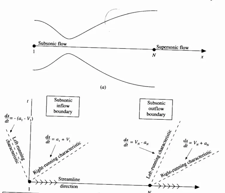
From the above fig, point 1 is the inflow boundary and point N is the outflow boundary. At point 1, left running characteristic line flows out of domain to the left and right running characteristic line, stream line flows into the domain to the right. So, 3 boundary conditions must be specified at point 1 out of which one variable value must be fixed and other two variables are allowed to float.
Similarly, at point N, left running characteristic line, right running characteristic line, stream line flows ouside the domain to the right. So, 3 boundary conditions must be specified at point N, that are allowed to float.
At point 1,
Fixed boundary conditions - ρ(1) = 1, T(1) = 1
Variable boundary condition - v(1) = 2*v(2) - v(3)
At point N,
Variable boundary condition - v(N) = 2*v(N-1) - v(N-2)
ρ(N) = 2*ρ(N-1) - ρ(N-2)
T(N) = 2*T(N-1) - T(N-2)
The variable boundary conditions are extrapolated by using linear extrapolation.
MATLAB CODE - Non conservative form:
clc;
clear all;
close all;

nx1 = [31,61,151,301,601,1001,2001,5001,6001,7001,8001,9001,10001,15001,20001,25001,30001];

%non-conservative form
for i = 1:length(nx1)
L = 3;  %length of nozzel
nx = nx1(i);    %no.of grid points in x-direction
x = linspace(0,L,nx);   %x-axis grid domain
dx = x(2)-x(1);  %grid size
nt = 1000; %time steps
dt = 0.001;
ghamma = 1.4;
throat = (nx+1)/2; %% middel node

%field variables initial conditions
rho = 1-0.3146*x;
T = 1-0.2314*x;
v = (0.1+1.09*x).*T.^0.5;

%area
A = 1+2.2*((x-1.5).^2);

for k = 1:nt   %time loop

    rho_old = rho;
    v_old = v;
    T_old = T;

    %time step calculation
        dt = min(0.5*dx./(T.^0.5+v));

    % predictor loop
    for j = 2:nx-1   %space loop
        dvdx = (v(j+1) - v(j))/dx;
        drho_dx = (rho(j+1) - rho(j))/dx;
        dlna_dx = log(A(j+1)/A(j))/dx;
        dTdx = (T(j+1) - T(j))/dx;

        %derivatives of field variables in predictor step
        drho_dt_predictor(j) = -rho(j)*dvdx - rho(j)*v(j)*dlna_dx - v(j)*drho_dx;
        dv_dt_predictor(j) = -v(j)*dvdx - (1/ghamma)*(dTdx + drho_dx*(T(j)/rho(j)));
        dT_dt_predictor(j) = -v(j)*dTdx - (ghamma-1)*T(j)*(dvdx + v(j)*dlna_dx);

        %solution update in predictor step
        rho(j) = rho(j) + drho_dt_predictor(j)*dt;
        v(j) = v(j) + dv_dt_predictor(j)*dt;
        T(j) = T(j) + dT_dt_predictor(j)*dt;

    end


    %corrector step
    for j = 2:nx-1   %space loop
        dvdx = (v(j) - v(j-1))/dx;
        drho_dx = (rho(j) - rho(j-1))/dx;
        dlna_dx = log(A(j)/A(j-1))/dx;
        dTdx = (T(j) - T(j-1))/dx;

        %derivatives of field variables in corrector time step
        drho_dt_corrector(j) = -rho(j)*dvdx - rho(j)*v(j)*dlna_dx - v(j)*drho_dx;
        dv_dt_corrector(j) = -v(j)*dvdx - (1/ghamma)*(dTdx + drho_dx*(T(j)/rho(j)));
        dT_dt_corrector(j) = -v(j)*dTdx - (ghamma-1)*T(j)*(dvdx + v(j)*dlna_dx);

    end

    %average derivative of field variables
    drho_dt_avg = 0.5*(drho_dt_predictor + drho_dt_corrector);
    dv_dt_avg = 0.5*(dv_dt_predictor + dv_dt_corrector);
    dT_dt_avg = 0.5*(dT_dt_predictor + dT_dt_corrector);

    %%final solution update
    for j = 2:nx-1
    rho(j) = rho_old(j) + drho_dt_avg(j)*dt;
    v(j) = v_old(j) + dv_dt_avg(j)*dt;
    T(j) = T_old(j) + dT_dt_avg(j)*dt;
    end

    %boundary conditions
    %inflow
    v(1) = 2*v(2) - v(3);

    %outflow
    v(nx) = 2*v(nx-1)-v(nx-2);
    rho(nx) = 2*rho(nx-1)-rho(nx-2);
    T(nx) = 2*T(nx-1)-T(nx-2);

    M = v./sqrt(T);   %%mach number
    p = rho.*T;    %pressure value
    m = rho.*A.*v; %mass flow rate

    v_throat(k) = v(throat);
    rho_throat(k) = rho(throat);
    p_throat(k) = p(throat);
    M_throat(k) = M(throat);
    T_throat(k) = T(throat);


if i==1
    figure(1)
    if k==1
        plot(x,m)
        hold on
        xlabel('nozzel length')
        ylabel('mass flow rate')
        title('Variation of mass flow rate at different time steps')
    elseif k==50
        plot(x,m)
    elseif k==100
        plot(x,m)
    elseif k==150
        plot(x,m)
    elseif k==250
        plot(x,m)
    elseif k==500
        plot(x,m)
   elseif k==1000
        plot(x,m,'LineWidth',2)
legend('1st timestep','50th timestep','100th timestep','150h timestep','250th timestep','500th timestep','1000th timestep')
    end
end

end

vel_throat_steady(i) = v_throat(1000);
rho_throat_steady(i) = rho_throat(1000);
T_throat_steady(i) = T_throat(1000);

if i==1
hold off
figure(2)
subplot(5,1,1)
    plot(x,v)
    xlabel('nozzel length')
    ylabel('velocity')
    title('variation of field varaibles inside the nozzel at steady state')
    subplot(5,1,2)
    plot(x,rho)
    xlabel('nozzel length')
    ylabel('density')
    subplot(5,1,3)
    plot(x,T)
    xlabel('nozzel length')
    ylabel('Temperature')
    subplot(5,1,4)
    plot(x,p)
    xlabel('nozzel length')
    ylabel('pressure')
    subplot(5,1,5)
    plot(x,M)
    xlabel('nozzel length')
    ylabel('Mach number')

figure(3)
    subplot(5,1,1)
    plot(v_throat)
    xlabel('no.of iterations')
    ylabel('velocity')
    title('variation of field varaibles at throat')
    subplot(5,1,2)
    plot(rho_throat)
    xlabel('no.of iterations')
    ylabel('density')
    subplot(5,1,3)
    plot(T_throat)
    xlabel('no.of iterations')
    ylabel('Temperature')
    subplot(5,1,4)
    plot(p_throat)
    xlabel('no.of iterations')
    ylabel('pressure')
    subplot(5,1,5)
    plot(M_throat)
    xlabel('no.of iterations')
    ylabel('Mach number')
end


end

figure(4)
subplot(3,1,1)
plot(nx1,vel_throat_steady,'-o')
xlabel('no.of grid points')
ylabel('velocity at steady state condition')
subplot(3,1,2)
plot(nx1,rho_throat_steady,'-o')
xlabel('no.of grid points')
ylabel('density at steady state condition')
subplot(3,1,3)
plot(nx1,T_throat_steady,'-o')
xlabel('no.of grid points')
ylabel('Temperature at steady state condition')
2) Non - Conservative form -
The governing equations are expressed in non dimensional forms, in terms of solution vector (U), flux vector (F), source term (J).
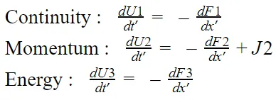
where,
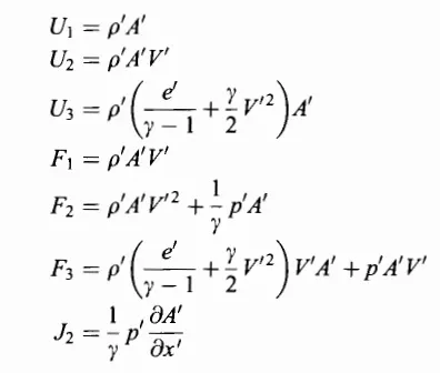
Initial conditions -
The initial conditions are chosen in such a manner that it replicates the flow field. So, as the flow expands through the nozzle, the pressure and temperature decreases and velocity increases and these are represented in the below equations.
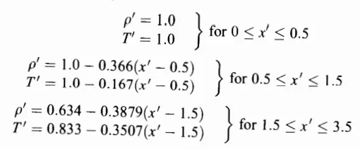
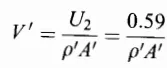
Since, in conservative form the governing equations is slightly more sensitive compared to non-conservative form, the initial conditions are slightly more precise.
Boundary conditions -
At point 1,


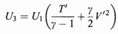
Since, v' floats the U3 value must be updated
At point N,
U1(N) = 2*U1(N-1) - U1(N-2)
U2(N) = 2*U2(N-1) - U2(N-2)
U3(N) = 2*U3(N-1) - U3(N-2)
MATLAB CODE - Conservative form:
clc
clear all
close all

nx1 = [31,61,151,301,601,1001,2001,5001,6001,7001,8001,9001,10001,15001,20001,25001,30001];

%conservative form
for i = 1:length(nx1)
L = 3;  %length of nozzel
nx = nx1(i);    %no.of grid points in x-direction
x = linspace(0,L,nx);   %x-axis grid domain
dx = x(2)-x(1);  %grid size
nt = 6000; %time steps
ghamma = 1.4;
throat = (nx+1)/2; %% middel node

%area
A = 1+2.2*(x-1.5).^2;

%field variable initial conditions
for z = 1:nx
    if x(z) < 0.5
        rho(z) = 1;
        T(z) = 1;
    elseif (x(z) >= 0.5 && x(z) < 1.5)
        rho(z) = 1-0.366*(x(z)-0.5);
        T(z) = 1-0.167*(x(z)-0.5);
    elseif (x(z) >= 1.5 && x(z) < 3.5)
        rho(z) = 0.634 - 0.3879*(x(z)-1.5);
        T(z) = 0.833 - 0.3507*(x(z)-1.5);
    end
end

v = 0.59./(rho.*A);  %%velocity initial condition

U1 = rho.*A;
U2 = rho.*A.*v;
U3 = rho.*((T/(ghamma-1)) + (ghamma/2)*v.^2).*A;

for k = 1:nt  %time loop
    U1_old = U1;
    U2_old = U2;
    U3_old = U3;

    dt = min(0.5*dx./(T.^0.5+v));  %%time step

        %flux vectors
        F1 = U2;
        F2 = U2.^2./U1 + ((ghamma-1)/ghamma)*(U3-(ghamma/2)*U2.^2./U1);
        F3 = ghamma*U2.*U3./U1 - (ghamma*(ghamma-1)/2)*U2.^3./U1.^2;


    for j = 2:nx-1 %%predictor loop

        %source vectors
        J2 = ((ghamma-1)/ghamma)*(U3(j)-(ghamma/2)*U2(j)^2/U1(j))*(log(A(j+1)/A(j))/dx);

        %derivatives in predictor time step
        du1_dt_predictor(j) = -(F1(j+1)-F1(j))/dx;
        du2_dt_predictor(j) = -(F2(j+1)-F2(j))/dx + J2;
        du3_dt_predictor(j) = -(F3(j+1)-F3(j))/dx;

        %Solution update in predictor loop
        U1(j) = U1(j) + du1_dt_predictor(j)*dt;
        U2(j) = U2(j) + du2_dt_predictor(j)*dt;
        U3(j) = U3(j) + du3_dt_predictor(j)*dt;
    end


    for j = 2:nx-1    %%%corrector loop

        J2 = ((ghamma-1)/ghamma)*(U3(j)-(ghamma/2)*U2(j)^2/U1(j))*(log(A(j)/A(j-1))/dx);
        %flux vectors
        F1(j) = U2(j);
        F2(j) = U2(j)^2/U1(j) + ((ghamma-1)/ghamma)*(U3(j)-(ghamma/2)*U2(j)^2/U1(j));
        F3(j) = ghamma*U2(j)*U3(j)/U1(j) - (ghamma*(ghamma-1)/2)*U2(j)^3/U1(j)^2;

        %derivatives in corector loop
        du1_dt_corrector(j) = -(F1(j)-F1(j-1))/dx;
        du2_dt_corrector(j) = -(F2(j)-F2(j-1))/dx + J2;
        du3_dt_corrector(j) = -(F3(j)-F3(j-1))/dx;
    end


        %average of the derivatives
        du1_dt_avg = 0.5*(du1_dt_predictor + du1_dt_corrector);
        du2_dt_avg = 0.5*(du2_dt_predictor + du2_dt_corrector);
        du3_dt_avg = 0.5*(du3_dt_predictor + du3_dt_corrector);

        %%final solution update
        for j = 2:nx-1
            U1(j) = U1_old(j) + du1_dt_avg(j)*dt;
            U2(j) = U2_old(j) + du2_dt_avg(j)*dt;
            U3(j) = U3_old(j) + du3_dt_avg(j)*dt;
        end


        %%boundary conditions
        %inflow
        U1(1) = A(1);
        U2(1) = 2*U2(2) - U2(3);
        U3(1) = U1(1)*(T(1)/(ghamma-1) + (ghamma/2)*v(1)^2);

        %outflow
        U1(nx) = 2*U1(nx-1) - U1(nx-2);
        U2(nx) = 2*U2(nx-1) - U2(nx-2);
        U3(nx) = 2*U3(nx-1) - U3(nx-2);

        rho = U1./A;   %density
        v = U2./U1;    %velocity
        T = (ghamma-1)*(U3./U1 - (ghamma/2)*v.^2);  %Temperature

        M = v./sqrt(T);   %%mach number
        p = rho.*T;    %pressure value
        m = rho.*A.*v; %mass flow rate

        v_throat(k) = v(throat);
        rho_throat(k) = rho(throat);
        p_throat(k) = p(throat);
        M_throat(k) = M(throat);
        T_throat(k) = T(throat);

 if i ==1
    figure(1)
    if k==1
        plot(x,m)
        hold on
        xlabel('nozzel length')
        ylabel('mass flow rate')
        title('Variation of mass flow rate at different time steps')
    elseif k==50
        plot(x,m)
    elseif k==100
        plot(x,m)
    elseif k==150
        plot(x,m)
    elseif k==250
        plot(x,m)
    elseif k==500
        plot(x,m)
   elseif k==1000
        plot(x,m,'LineWidth',2)
legend('1st timestep','50th timestep','100th timestep','150h timestep','250th timestep','500th timestep','1000th timestep')
    end
 end
end

vel_throat_steady(i) = v_throat(1000);
rho_throat_steady(i) = rho_throat(1000);
T_throat_steady(i) = T_throat(1000);

if i==1
hold off
figure(2)
subplot(5,1,1)
    plot(x,v)
    xlabel('nozzel length')
    ylabel('velocity')
    title('variation of field varaibles inside the nozzel at steady state')
    subplot(5,1,2)
    plot(x,rho)
    xlabel('nozzel length')
    ylabel('density')
    subplot(5,1,3)
    plot(x,T)
    xlabel('nozzel length')
    ylabel('Temperature')
    subplot(5,1,4)
    plot(x,p)
    xlabel('nozzel length')
    ylabel('pressure')
    subplot(5,1,5)
    plot(x,M)
    xlabel('nozzel length')
    ylabel('Mach number')

figure(3)
    subplot(5,1,1)
    plot(v_throat)
    xlabel('no.of iterations')
    ylabel('velocity')
    title('variation of field varaibles at throat')
    subplot(5,1,2)
    plot(rho_throat)
    xlabel('no.of iterations')
    ylabel('density')
    subplot(5,1,3)
    plot(T_throat)
    xlabel('no.of iterations')
    ylabel('Temperature')
    subplot(5,1,4)
    plot(p_throat)
    xlabel('no.of iterations')
    ylabel('pressure')
    subplot(5,1,5)
    plot(M_throat)
    xlabel('no.of iterations')
    ylabel('Mach number')
end

end

figure(4)
subplot(3,1,1)
plot(nx1,vel_throat_steady,'-o')
xlabel('no.of grid points')
ylabel('velocity at steady state condition')
subplot(3,1,2)
plot(nx1,rho_throat_steady,'-o')
xlabel('no.of grid points')
ylabel('density at steady state condition')
subplot(3,1,3)
plot(nx1,T_throat_steady,'-o')
xlabel('no.of grid points')
ylabel('Temperature at steady state condition')
RESULTS -
NOTE - The output / field variables are expressed in non dimensional form.
1)Non-conservative form -
Initially, the flow is unsteady. The fig1 shows the variation of mass flow rate inside the nozzel at different time steps. It is observed that initially as the flow is unsteady the mass flow rate is not uniform inside the nozzle. Once, the steady-state is reached, the flow is stable. In 250th time step, the flow almost reaches steady-state and in 1000th time step, steady-state is already reached. The mass flow rate at steady-state is 0.587 units as these are expressed in non-dimensional form.
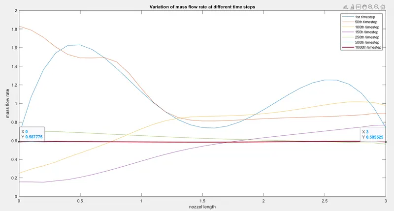
FIG 1 - VARIATION OF MASS FLOW RATE
The fig2 shows the variation of field variables such as velocity, density, temperature, mach number inside the nozzle once steady state is reached. It is observed that at steady,
At inlet, v = 0.0987, ρ = 1, T = 1, P = 1
At outlet, v = 1.8617, ρ = 0.0528, T = 0.3082, P = 0.0162
Since, as flow is expanding, through the nozzle, velocity increases and pressure, temperature, density decreases.
At x=1.5, mach number is ~1, which indicates sonic flow. At x < 1.5, mach number < 1 which indicates sunsonic flow
At x>1.5 mach number <1 which indicates supersonic flow.
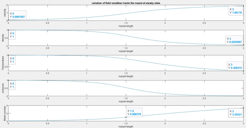
FIG 2 - VARIATION OF FIELD VARIABLES INSIDE THE NOZZEL AT STEADY STATE
The fig3 shows the variation of field variables such as velocity, density, temperature, mach number at throat section inside the nozzle.
It is observed that fluctuations in filed variables is more till 300th time step and afterwards it reaches to staedy state after 500th time step.
| 300th time step | 1000th time step | |
| Velocity | 0.9190 | 0.9140 |
| Density | 0.6595 | 0.6386 |
| Temperature | 0.8486 | 0.8364 |
| Pressure | 0.5595 | 0.5342 |
| Mach number | 0.9964 | 0.9993 |
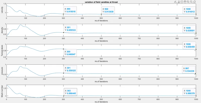
FIG 3 - VARIATION OF FIELD VARIABLES AT THROAT SECTION
The fig 4 shows the variation of the throat section flow variables when the grid size is changed.It is known that, the accuracy of the numerical method increases as the grid size decreases. In other words, fine mesh gives accurate results compared to coarse mesh. Here, grid independence test is performed so that until which mesh size, the results gets affected is validated. It is observed that as no.of grid points > 15000, there is no much change in the final solution. So, it is advisable not to make mesh size too fine as it increases the computational cost.
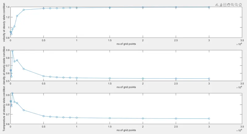
FIG 4 - Field variables v/s no.of grid points
2) Conservative form -
The fig5 shows the variation of mass flow rate inside the nozzel at different time steps. It is observed that initially as the flow is unsteady the mass flow rate is not uniform inside the nozzle. Once, the steady-state is reached, the flow is stable. In 250th time step, there is not much variation in the the flow and in 1000th time step, steady-state is reached. The mass flow rate at steady-state is 0.587 units as these are expressed in non-dimensional form.
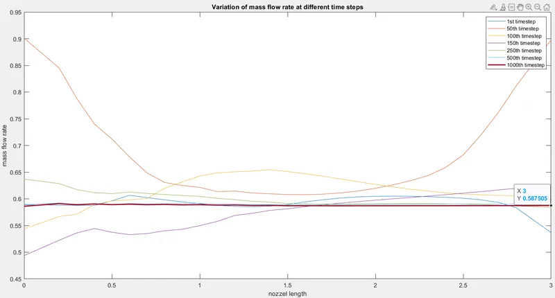
FIG 5 - VARIATION OF MASS FLOW RATE
The fig6 shows the variation of field variables such as velocity, density, temperature, mach number inside the nozzle once steady state is reached. It is observed that at steady,
At inlet, v = 0.0985, ρ = 1, T = 1.00004, P = 1.00004
At outlet, v = 1.8659, ρ = 0.0529, T = 0.3056, P = 0.0161
Since, as flow is expanding, through the nozzle, velocity increases and pressure, temperature, density decreases.
Theoritically, the min area of the nozzle is at x=1.5, but due to inertia effect, the min flow area doesn't exactly occur at x =1.5 . In the fig, it is observed that M=1 occurs at 1.5 < x < 1.6, which indicates the sonic flow exists in that particular region where M = 1.
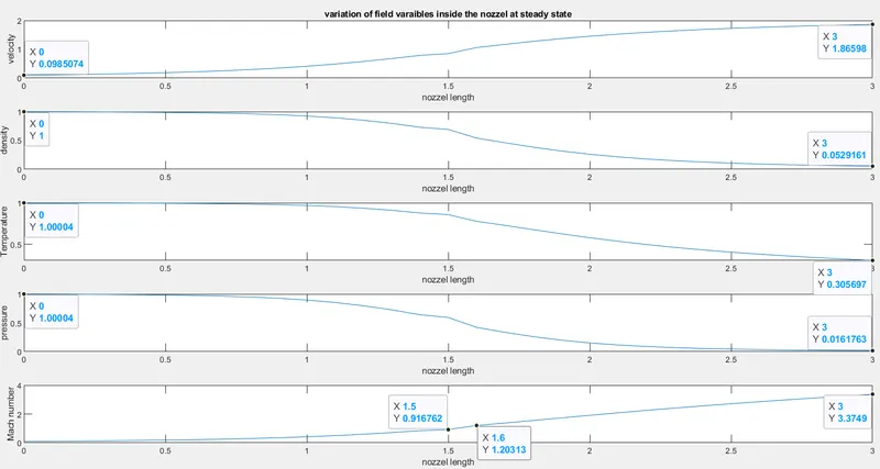
FIG 6 - VARIATION OF FIELD VARIABLES INSIDE THE NOZZEL AT STEADY STATE
The fig7 shows the variation of field variables such as velocity, density, temperature, mach number at throat section inside the nozzle. Sice, the conservative form is more sensitive, it takes more time steps in order to converge. It is observed that fluctuations in filed variables is more till 500th time step and afterwards it reaches to staedy state after 800th time step.
| 800th time step | 1000th time step | |
| Velocity | 0.8515 | 0.8492 |
| Density | 0.6898 | 0.6912 |
| Temperature | 0.8574 | 0.8580 |
| Pressure | 0.5915 | 0.5931 |
| Mach number | 0.9195 | 0.9167 |
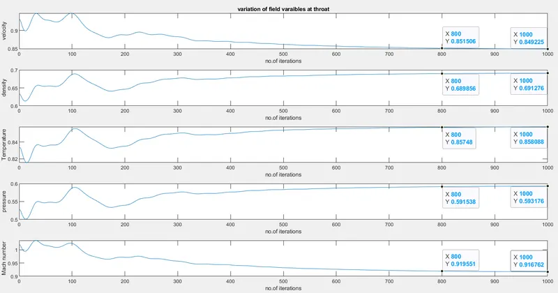
FIG 7 - VARIATION OF FIELD VARIABLES AT THROAT SECTION
The fig 8 shows the variation of the throat section flow variables when the grid size is changed.It is known that, the accuracy of the numerical method increases as the grid size decreases. In other words, fine mesh gives accurate results compared to coarse mesh. Here, grid independence test is performed so that until which mesh size, the results gets affected is validated. It is observed that as no.of grid points > 15000, there is no much change in the final solution. So, it is advisable not to make mesh size too fine as it increases the computational cost.
In reality, gird independence test, the no.of grid points can be obtained when percentage change in the output values is < 5% so that accurate results are obtained with reasonable computational cost.
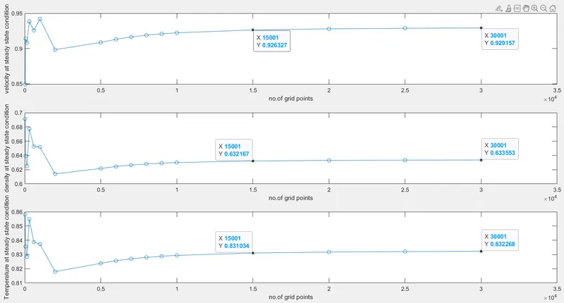
FIG 8 - Field variables v/s no.of grid points
In fig 9, shows the mass flow rate of conservative form and non conservative form throughout the nozzle length at 1400th iteration with no.of grid points as 31. As discussed above in both the forms steady state is reached within 1000th iteration. The analytical mass flow rate at steady state is 0.579. It is observed that conservative form shows less oscillations compared to non-conservative form. The conservative form solution is much closer to the analytical solution compared to non-conservative form solution.
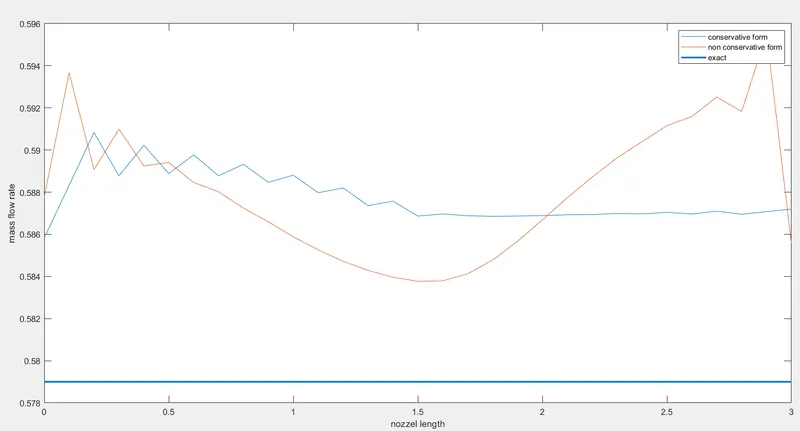
FIG 9 - Conservative form v/s non-conservative form
The Fig 10 also shows same result compared to fig 9. The only difference is in fig 9, the J2 value is calculated by using
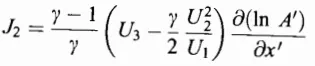
And in fig 10, the J2 value is calculated by using the following equation
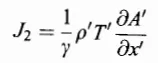 .
.
Since in fig 10, simpler version of J2 is used, means J2 is calculated by using the primitive (or) flow field variables, much accurate results of mass flow rate is obtained compared to fig9.
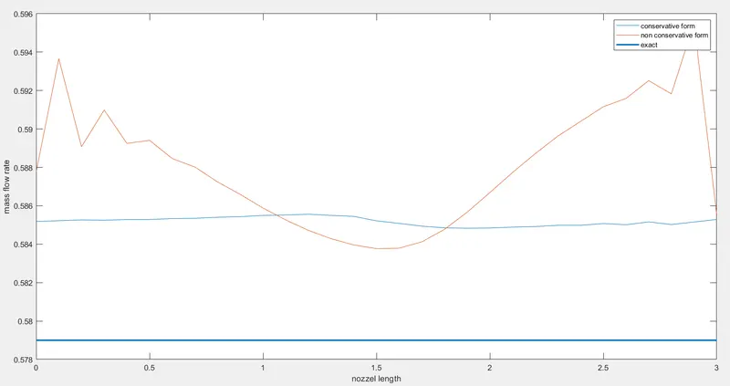
FIG 10 - Conservative form v/s non-conservative form_J2 with primitive variables
CONCLUSION:
The conservative form shows accurate results compared to non conservative form.