Week 7 - Simulation of a 1D Super-sonic nozzle flow simulation using Macormack Method
Simulation of 1D supersonic nozzle using Macormack technique
It is widely used discretization method for solving hyperbolic partial differential equations.
We are considering the steady state isentropic flow throght convergent-divergent nozzle . The flow is from the reservoir. The flow expands isentropically to supersonic speeds at nozzle exit where we have properties like pressure, temperature, Mach no, velocity. Flow is subsonic at the convergent section of the nozzle. Its Mach no. is 1 hat the thorat i.e. its sonic at throat.
Even if the flow is 2 dimensional flow, we make the assumption that flow properties vary only with x, so its assumed that flow properties are uniform across any given section. Such is called as Quasi-1D flow.
We will solve this by setting up time marching solutions, finite difference solution for Quasi 1D nozzle flow. The governing equations like continuity, momentum and energy equations are written in terms of PDE's suitable for time marching solution.
We will solve this problem in two forms namely conservative and non-conservative.
Optimum criterion for dt, time steps, Courant number, grid point is taken.
Equations for Non-conservative form :
1) Continuity equation
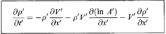
2) Momentum equation
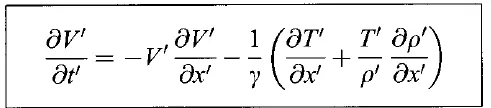
3) Energy equation

Equations for conservative form :
1) Continuity equation
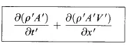
2) momentum eqaution
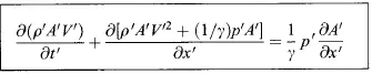
3)Enrgy equaiton

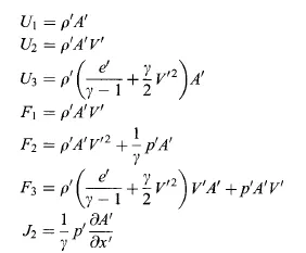
Let us define elements of solution vector U, the flux vector F and source term J as below,
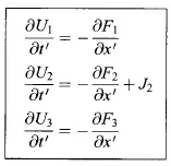
With these, the governing equations are wroteen as ,
The main code for Non-conservative form is as below,
clear all
close all
clc

% inputs
L = 3; % Length of the nozzle
n =31 ;  % no. of grid points/ nodes
x = linspace(0, L, n);  %domain of points
dx = x(2)- x(1); % grid size

% Constants
gamma =1.4;

% Solution of nozzle flow of Non-conservative form using MacCormack technique

% Calculate initial profiles
rho = 1 - 0.3146* x ;
t = 1-0.2314* x; % t = temperature
v = (0.1+1.09*x).*t.^0.5;
a = 1+2.2*(x-1.5).^2 ;
v_old = v;
rho_old = rho;
t_old = t;
% Time steps
nt = 700;

% Finding dt as per CFL criterion
  C = 0.5;
for q = 1:length(x)

    A =t.^0.5 ;
    dt(q) = (C*dx)/(A(q)+ v(q));
end
dt = min(dt);

% outer time loop

for k =1:nt

    v_old = v;
    rho_old = rho;
    t_old = t;

    %Predictor step

    % continuity equation

    for i = 2:n-1
      %  drho_dt_p = -rho(i)*((v(i+1)-v(i))/dx)-(rho(i)*v(i)*(log(a(i+1)-log(a(i)))/dx))-(v(i)*((rho(i+1)-rho(i))/dx));
       dvdx = (v(i+1)-v(i))/dx ;
       drhodx = (rho(i+1)-rho(i))/dx ;
       dtdx = (t(i+1)-t(i))/dx ;
       dlog_a_dx = (log(a(i+1))-log(a(i)))/dx ;

        % continuity equation

       drho_dt_p(i) = -rho(i)* dvdx -rho(i)*v(i)*dlog_a_dx- v(i)*drhodx;

       % momentum equation

       dvdt_p(i) = -v(i)*dvdx -(1/gamma)* (dtdx + (t(i)/rho(i))*drhodx);

       % Energy equation

       dTdt_p(i) = -v(i)*dtdx-(gamma-1)*t(i)*(dvdx+v(i)*dlog_a_dx);

       % solution update
       v(i) = v(i) + dvdt_p(i) * dt;
       rho(i) = rho(i) + drho_dt_p(i)*dt;
       t(i) = t(i) + dTdt_p(i)*dt

    end

    % Corrector method
    for i = 2:n-1
      %  drho_dt_p = -rho(i)*((v(i+1)-v(i))/dx)-(rho(i)*v(i)*(log(a(i+1)-log(a(i)))/dx))-(v(i)*((rho(i+1)-rho(i))/dx));
       dvdx = (v(i)-v(i-1))/dx ;
       drhodx = (rho(i)-rho(i-1))/dx ;
       dtdx = (t(i)-t(i-1))/dx ;
       dlog_a_dx = (log(a(i))-log(a(i-1)))/dx ;

        % continuity equation

       drho_dt_c(i) = -rho(i)* dvdx - rho(i)*v(i)*dlog_a_dx- v(i)*drhodx;

       % momentum equation

       dvdt_c(i) = -v(i)*dvdx -(1/gamma)* (dtdx + (t(i)/rho(i))*drhodx );

       % Energy equation

       dTdt_c(i) = -v(i)*dtdx-(gamma-1)*t(i)*(dvdx+v(i)*dlog_a_dx);

    end

    % Finding average time derivative

    drho_dt = (drho_dt_p + drho_dt_c)/2;
    dvdt = (dvdt_p + dvdt_c)/2;
    dTdt = (dTdt_p + dTdt_c)/2 ;


    % Final solution update
    for j = 2: n-1
        rho(j) = rho_old(j) + drho_dt(j)*dt ;
        v(j) = v_old(j) + dvdt(j)*dt;
        t(j) = t_old(j) + dTdt(j)*dt;
    end

    % Apply boundary condiitons
    % Inlet boundary condition
    v(1) = 2*v(2) - v(3);

    % Pressure and temperature are stagnation values as constants

    % outlet
    v(n) = 2*v(n-1)-v(n-2);
    rho(n) = 2*rho(n-1)-rho(n-2);
    t(n) = 2*t(n-1)-t(n-2);

    % Final values
    p = rho.* t;
    M = v./t.^0.5;
    mdot = rho.* a.* v ;

    % storing values in all time steps
    v_non(k,:) = v ;
    t_non(k,:) = t;
    rho_non(k,:) = rho;
    p_non (k,:)= p;
    M_non(k,:) = M;
    mdot_non(k,:) = mdot;

% Time wise variation of primetive variables

figure (1)
subplot(2,2,1);
plot(x,rho, 'linewidth', 1, 'color', 'r');
title(sprintf('Density Distribution at time step t = %d', k))
xlabel('Nozzle length')
ylabel('Density')
grid on

subplot(2,2,2);
plot(x,t, 'linewidth', 1, 'color', 'r');
title(sprintf('Temperature Distribution at time step t = %d', k))
xlabel('Nozzle length')
ylabel('Temperature')
grid on

subplot(2,2,3);
plot(x,p, 'linewidth', 1, 'color', 'r');
title(sprintf('Pressure Distribution at time step t = %d', k))
xlabel('Nozzle length')
ylabel('Pressure')
grid on

subplot(2,2,4);
plot(x,M, 'linewidth', 1, 'color', 'r');
title(sprintf('Mach number Distribution at time step t = %d', k))
xlabel('Nozzle length')
ylabel('Temperature')
grid on

sgtitle('Time wise distribution of Primitive variables')

end

% Property variation of primitive variables at throat of nozzle

figure (2)
subplot(2,2,1)
plot((1:nt),rho_non(:,16));
title(sprintf('Density discretisation at time step= %d',k));
xlabel('No. of time steps')
ylabel('Density')
grid on

subplot(2,2,2)
plot((1:nt),t_non(:,16));
title(sprintf('Temperature discretisation at time step= %d',k));
xlabel('No. of time steps')
ylabel('Temperature')
grid on

subplot(2,2,3)
plot((1:nt),p_non(:,16));
title(sprintf('Pressure discretisation at time step= %d',k));
xlabel('No. of time steps')
ylabel('Pressure')
grid on

figure (2)
subplot(2,2,4)
plot((1:nt),M_non(:,16));
title(sprintf('Mach number discretisation at time step= %d',k));
xlabel('No. of time steps')
ylabel('Mach no.')
grid on

sgtitle('time wise variation of Primitive variables at nozzle throat');
Results for the above code are,
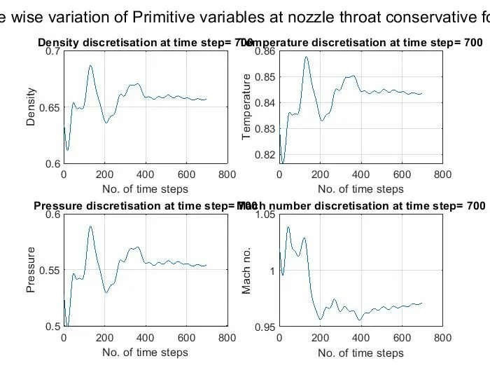
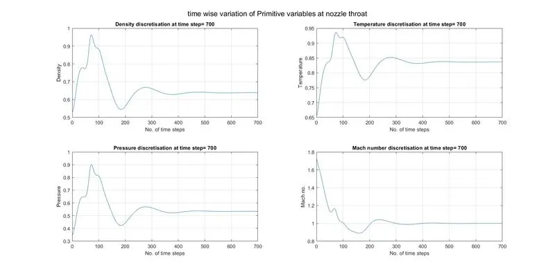
1) The variation of rho, T, p and Mach no. at nozzle throat is plotted vs time number of time steps.Abscissa starts from 0 and goes upto 700. The large changes are seen at initial time steps and with the increase in time steps as it approaches steady state the changes becomes smaller and at about 400 time step, it becomes stable.
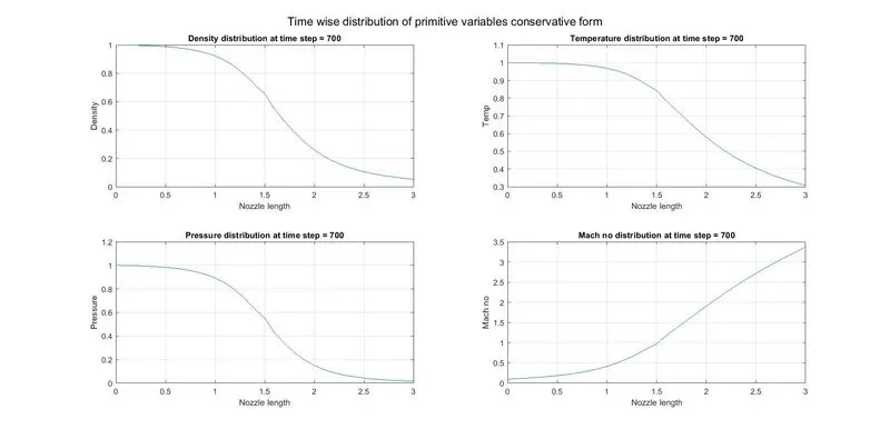
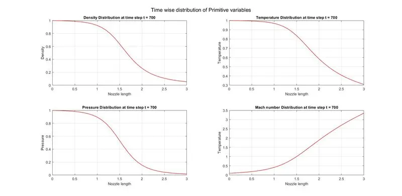
2) Steady state profile of the primititive variables are shown below, we can see that when the flow becomes steady the density, pressure and temperature at the inlet is unity and the velocity at the inlet very less and as the flow approaches the nozzle throat the desnity, pressre and temperature decreases and speed increases.
2) Solution of conservative form by Maccormack technique
clear all
close all
clc

% inputs
L = 3; % Length of the nozzle
n =31 ;  % no. of grid points/ nodes
x = linspace(0, L, n);  %domain of points
dx = x(2)- x(1); % grid size

% Constants
gamma =1.4;


% solution of conservative form using Maccormack mthod

% initial condition

for ct = 1:n
   if ((x(ct)>=0) && (x(ct)<=0.5))
    rhoc(ct)=1;
    tc(ct)=1;


    elseif ((x(ct)<1.5) && (x(ct)>0.5))
        rhoc(ct)=1-0.366*(x(ct)-0.5);
        tc(ct)=1-0.167*(x(ct)-0.5);
     elseif ((x(ct)>=1.5) && (x(ct)<=3.5))
        rhoc(ct)=0.634-0.3879*(x(ct)-1.5);
        tc(ct)=0.833-0.03507*(x(ct)-1.5);
    end
end

% calculate initial profiles
a = 1+2.2*(x-1.5).^2 ;
pc = rhoc.*tc;
% u2= 0.59.* ones(1,n);
vc=0.59./(rhoc.*a);
% vc = u2./(rhoc.*a);
% u2old =u2;
% solution vector
u1= rhoc.*a;
u2 = rhoc.*a.*vc ;
u3 = rhoc.*(tc./(gamma-1)+(gamma/2)*vc.^2).*a;
% finding dt value as per CFL criterion
for q = 1:length(x)
    A = tc.^0.5;
    C= 0.5;
    dt(q)= (C*dx)/(A(q)+vc(q));
end
dt =min(dt)


% time steps
ntc = 700;

    u1_old = u1;
    u2_old = u2;
    u3_old = u3;
% outer time loop

for k =1: ntc

    u1_old = u1;
    u2_old = u2;
    u3_old = u3;

    %flux terms
    f1 = u2;
    f2=(u2.^2)./u1+((gamma-1)/gamma)*(u3-(gamma/2)*(u2.^2)./u1);
     f3=(gamma*u2.*u3)./u1-((gamma*(gamma-1)/2)*(u2.^3)./u1.^2);

%     rhoc = u1./a;
%     tc= (gamma-1)*((u3./u1)-((gamma/2)*(u2./u1).^2));

    % source term


    % predictor method
    for j= 2:n-1
        j2(j)=(1/gamma)*rhoc(j)*tc(j)*(a(j+1)-a(j))/dx;
         % continuity equation
         du1_dt_p(j) = -(f1(j+1)-f1(j))/dx;

         % momentum equation
         du2_dt_p(j)= -(f2(j+1)-f2(j))/dx + j2(j);

         % energy equation
         du3_dt_p(j) = -(f3(j+1)-f3(j))/dx ;

         % solutoion update

         u1(j)= u1(j)+ du1_dt_p(j)*dt;
         u2(j)= u2(j)+ du2_dt_p(j)*dt;
         u3(j)= u3(j)+ du3_dt_p(j)*dt;

    end


    % corrector method
rhoc=u1./a;
    v=u2./u1;
    tc=(gamma-1)*((u3./u1)-(gamma/2)*vc.^2);
    %flux terms
   f1 = u2;
    f2=(u2.^2)./u1+((gamma-1)/gamma)*(u3-(gamma/2)*(u2.^2)./u1);
     f3=(gamma*u2.*u3)./u1-((gamma*(gamma-1)/2)*(u2.^3)./u1.^2);

%     rhoc = u1./a;
%     tc= (gamma-1)*((u3./u1)-((gamma/2)*(u2./u1).^2));

    % source term


    % corrector method
    for j= 2:n-1
j2(j)=(1/gamma)*rhoc(j)*tc(j)*(a(j)-a(j-1))/dx;

         % continuity equation
         du1_dt_c(j) = -(f1(j)-f1(j-1))/dx;

         % momentum equation
         du2_dt_c(j)= -((f2(j)-f2(j-1))/dx)+j2(j);

         % energy equation
         du3_dt_c(j) = -(f3(j)-f3(j-1))/dx;

    end

    du1_dt = 0.5*(du1_dt_p + du1_dt_c);
    du2_dt = 0.5*(du2_dt_p + du2_dt_c);
    du3_dt = 0.5*(du3_dt_p + du3_dt_c);

    % final solution update

    for i= 2:n-1

        u1(i)= u1_old(i)+ du1_dt(i)*dt;
        u2(i)= u2_old(i)+ du2_dt(i)*dt;
        u3(i)= u3_old(i)+ du3_dt(i)*dt;

    end

    % apply boundary conditions
    % inlet
    u1(1)= rhoc(1).*a(1);
    u2(1)= 2*u2(2)-u2(3);
    vc(1)=u2(1)/u1(1);
%     tc(1)= (gamma-1)*((u3(1)/u1(1))-(gamma/2)*(u2(1)/u1(1))^2);
   u3(1)=u1(1)*(tc(1)/(gamma-1)+(gamma/2)*vc(1)^2);

    % outlet
    u1(n)= 2*u1(n-1)-u1(n-2);
    u2(n)= 2*u2(n-1)-u2(n-2);
    u3(n)= 2*u3(n-1)-u3(n-2);

    % Final value
    tc=(gamma-1)*((u3./u1)-(gamma/2)*vc.^2);
    rhoc = u1./a;
    vc = u2./u1;
        tc=(gamma-1)*((u3./u1)-(gamma/2)*vc.^2);
    pc= rhoc.*tc;

    % temp


    Mc = vc./(tc.^0.5);
    mdotc = rhoc.*vc.*a ;

        % storing values in all time steps at throat section
    v_con(k,:) = vc;
    t_con(k,:) = tc;
    rho_con(k,:) = rhoc;
    p_con(k,:) = pc;
    M_con(k,:) = Mc;
    mdot_con(k,:) = mdotc;

end

% steady state profile of primitive variables

figure(3);
subplot(2,2,1);
plot(x,rhoc);
title(sprintf('Density distribution at time step = %d',k));
xlabel('Nozzle length');
ylabel('Density');
grid on


subplot(2,2,2);
plot(x,tc);
title(sprintf('Temperature distribution at time step = %d',k));
xlabel('Nozzle length');
ylabel('Temp');
grid on


subplot(2,2,3);
plot(x,pc);
title(sprintf('Pressure distribution at time step = %d',k));
xlabel('Nozzle length');
ylabel('Pressure');
grid on


subplot(2,2,4);
plot(x,Mc);
title(sprintf('Mach no distribution at time step = %d',k));
xlabel('Nozzle length');
ylabel('Mach no');
grid on

sgtitle('Time wise distribution of primitive variables conservative form')

% compariosn graph

figure (4)
subplot(2,2,1)
plot((1:ntc),rho_con(:,16));
title(sprintf('Density discretisation at time step= %d',k));
xlabel('No. of time steps')
ylabel('Density')
grid on

subplot(2,2,2)
plot((1:ntc),t_con(:,16));
title(sprintf('Temperature discretisation at time step= %d',k));
xlabel('No. of time steps')
ylabel('Temperature')
grid on

subplot(2,2,3)
plot((1:ntc),p_con(:,16));
title(sprintf('Pressure discretisation at time step= %d',k));
xlabel('No. of time steps')
ylabel('Pressure')
grid on

subplot(2,2,4)
plot((1:ntc),M_con(:,16));
title(sprintf('Mach number discretisation at time step= %d',k));
xlabel('No. of time steps')
ylabel('Mach no.')
grid on

sgtitle('time wise variation of Primitive variables at nozzle throat conservative form');
Results: