Week 5.1 - Mid term project - Solving the steady and unsteady 2D heat conduction problem
This assignment is to solve two dimensional heat conduction equation in steady and transient state by discretizing the equation.
1) Transient state - implicit
Let us first consider transient state equation as below,
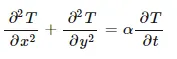 , where alpha is constant and no internal heat generation.
We discretize the space terms by central differencing scheme as below,
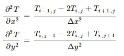
We discretize time domain by forward differencing scheme,
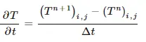
So the equation after discretization becomes,

 ,
, 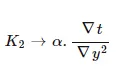 .
.
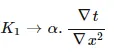
CFLx = K1 and CFLy = K2.
%% Code for Implicit method - unsteady/ Transient

clear all
close all
clc

%inputs
L = 1;
nx = 10; % no of nodes along x axis
ny = 10; % no of nodes along y axis
nt = 300;

x = linspace(0,L,nx);
y = linspace(0,L,ny);

alpha = 1.4 ; % thermal diffusivity

tolerance = 1e-4
dt = 0.001;

omega = 1.1;

T = 300 *ones(nx ,ny)

%Boundary conditions
T(1,:) = 600;
T(end,:) = 900;
T(:,1) = 400;
T(:,end) = 800;

dx = x(2) - x(1);
dy = dx;

[xx yy] = meshgrid(x, y)

% CFL values
k1 = alpha*(dt/ (dx^2));
k2 = alpha*(dt/ (dy^2));

% Assigning original values to T
T_old = T;
T_prev = T;


% Calculating 2D steady state heat conduction equation by Jacobi method

iter_no = input('Enter the iter number')
error = 9e9

% Jacobi method

if iter_no == 1
 % jacobi method
 % time loop

 jacobi_iter = 1;

for k = 1: nt
    error= 9e9
while (error > tolerance)

  % space loop

for i= 2: nx -1

for j= 2: ny-1

        term1 = 1/(1+(2*(k1))+(2*(k2)));
        term2 = k1*term1;
        term3 = k2*term1;

        H = (T_old(i-1,j)+T_old(i+1,j));
        V = (T_old(i,j-1)+T_old(i,j+1));

        T(i,j)= (term1* T_prev(i,j))+ (term2 * H)+ (term3 * V);

end
end

error = max( max(abs(T - T_old)));
T_old = T ;
jacobi_iter = jacobi_iter + 1;
end

T_prev = T;

figure(2)
contourf(x,y,T)
colorbar
clabel(contourf(x,y,T))
colormap(jet)

xlabel('X-axis')
ylabel('Y-axis')
text = sprintf('No. of iterations  = %d',jacobi_iter)
title(text)
pause(0.03)
end

end


% Gauss-Seidal method

if iter_no == 2
 % GS method
 % time loop

  GS_iter = 1;

for k = 1: nt
    error= 9e9
while (error > tolerance)

  % space loop

for i= 2: nx -1

for j= 2: ny-1

        term1 = 1/(1+(2*(k1))+(2*(k2)));
        term2 = k1*term1;
        term3 = k2*term1;

        H = (T(i-1,j)+T_old(i+1,j));
        V = (T(i,j-1)+T_old(i,j+1));

        T(i,j)= (term1* T_prev(i,j))+ (term2 * H)+ (term3 * V);

end
end

error = max( max(abs(T - T_old)));
T_old = T ;
GS_iter = GS_iter + 1;
end

T_prev = T;

figure(3)
contourf(x,y,T)
colorbar
clabel(contourf(x,y,T))
colormap(jet)

xlabel('X-axis')
ylabel('Y-axis')
text = sprintf('No. of iterations  = %d',GS_iter)
title(text)
pause(0.03)
end

end

% SOR method

omega = 1.1;
if iter_no == 3
 % Successive over relaxation method
 % time loop

 SOR_iter = 1;

for k = 1: nt
    error= 9e9
while (error > tolerance)

  % space loop

for i= 2: nx -1

for j= 2: ny-1

        term1 = 1/(1+(2*(k1))+(2*(k2)));
        term2 = k1*term1;
        term3 = k2*term1;

        H = (T(i-1,j)+T_old(i+1,j));
        V = (T(i,j-1)+T_old(i,j+1));

        Tgs(i,j)= (term1* T_prev(i,j))+ (term2 * H)+ (term3 * V);
        T(i,j) = (T_old(i,j)*(1-omega))+ (omega * Tgs(i,j));

end
end

error = max(max(abs(T_old - T)));
T_old = T ;
SOR_iter = SOR_iter + 1;
end

T_prev = T;

figure(4)
contourf(x,y,T)
colorbar
clabel(contourf(x,y,T))
colormap(jet)

xlabel('X-axis')
ylabel('Y-axis')
text = sprintf('No. of iterations  = %d',SOR_iter)
title(text)
pause(0.03)

end

end
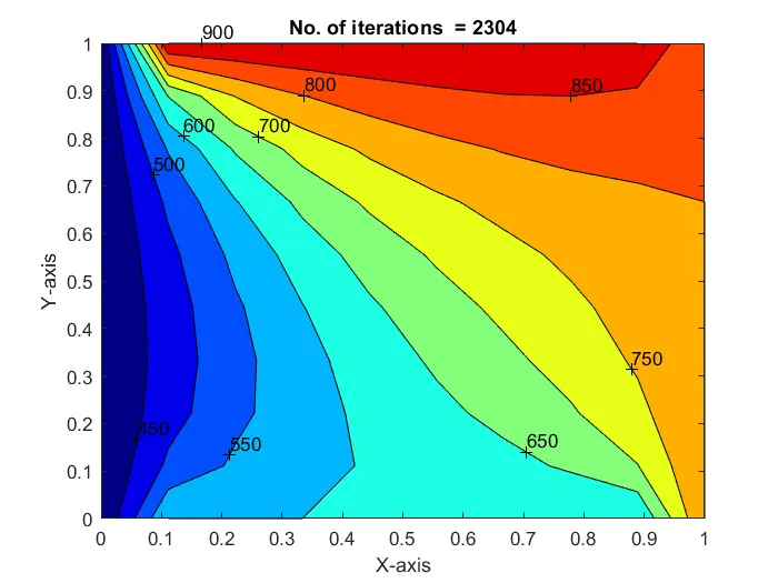
1) Jacobi method output
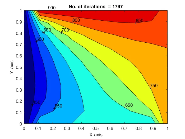
2) GS output
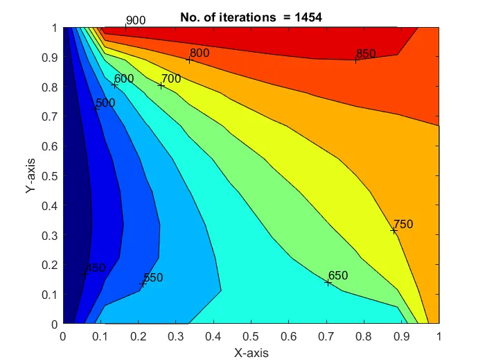
3) SOR output
2) Steady state -Implicit
Generalized 2D steady state equation is as below
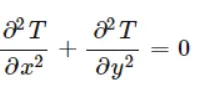
Let us discretize the equation as below,
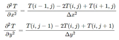
%% code for solving Steady state 2D equation

clear all
close all
clc

% Inputs
nx = 20;
ny = nx;
L = 1;

%Defining temperature at all grid points
T = 300 *ones(nx, ny);

%Boundary conditions
T(1,:) = 600;
T(end,:) = 900;
T(:,1) = 400;
T(:,end) = 800;

x = linspace(0, L, nx);
y = linspace(0, L, ny);

[xx yy] = meshgrid(x, y);

% Grid size in x and y direction
dx = x(2)- x(1) ;
dy = dx;

k = (2*(dx^2+dy^2))/ (dx^2 * dy^2);

% defining error and tolerance
error = 9e9;
tolerance = 1e-4 ;

T_old = T;

iter_no = input('Enter iteration type: ')

if (iter_no == 1)

% Jacobi method

  jacobi_iter = 1;

% convergence loop

while (error> tolerance)
    error = 9e9;

    for i = 2: nx -1
        for j= 2: ny-1

            term1 = ((T_old(i+1,j)+T_old(i-1,j))/(k* dx^2));
            term2 = ((T_old(i,j-1)+T_old(i,j+1))/(k* dy^2));

       T(i,j) = term1 + term2;

        end
    end
    error = max(max(abs( T - T_old))) ;
    T_old = T;

    jacobi_iter = jacobi_iter + 1;

end

end

    figure(3)
    contourf(x, y ,T)
    colorbar
    [a, b]= contourf(x,y,T);
    clabel(a,b);
    colormap(jet)
    xlabel('X-axis')
    ylabel('Y-axis')


    if (iter_no == 2)
         error = 9e9
   % Gauss -Seidal method
     GS_iter = 1;

    % convergence loop

while (error> tolerance)
    error = 9e9

    for i = 2: nx -1
        for j= 2: ny-1

            term1 = ((T_old(i+1,j)+T(i-1,j))/(k* dx^2));
            term2 = ((T(i,j-1)+T_old(i,j+1))/(k* dy^2));

       T(i,j) = term1 + term2;

        end
    end
    error = max(max(abs( T - T_old))) ;
    T_old = T;
    GS_iter = GS_iter + 1;

end

end

    figure(4)
    contourf(x, y ,T)
    colorbar
    [a, b]= contourf(x,y,T);
    clabel(a,b);
    colormap(jet)
    xlabel('X-axis')
    ylabel('Y-axis')


    if (iter_no == 3)

     % Successive over relaxation -steady state

     % SOR method

    omega = 1.1
    SOR_iter = 1;

    % convergence loop

while (error> tolerance)

    for i = 2: nx -1
        for j= 2: ny-1

            term1 = (T_old(i+1,j)+T(i-1,j))/(k* dx^2);
            term2 = (T(i,j-1)+T_old(i,j+1))/(k* dy^2);

       Tgs(i,j) = term1+ term2;
       T(i,j) =  (T_old(i,j)*(1-omega))+ (omega * Tgs(i,j));

        end
    end
    error = max(max(abs( T - T_old)));
    T_old = T;
    SOR_iter = SOR_iter + 1;

end

end

    figure(5)
    contourf(x, y ,T)
    colorbar
    [a, b]= contourf(x,y,T);
    clabel(a,b);
    colormap(jet)
    xlabel('X-axis')
    ylabel('Y-axis')

    text = sprintf('No. of iterations  = %d',SOR_iter)
    title(text)
Outputs :
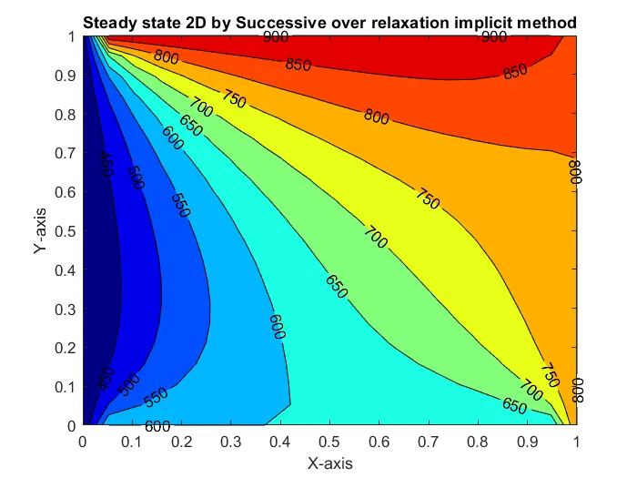
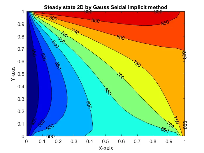
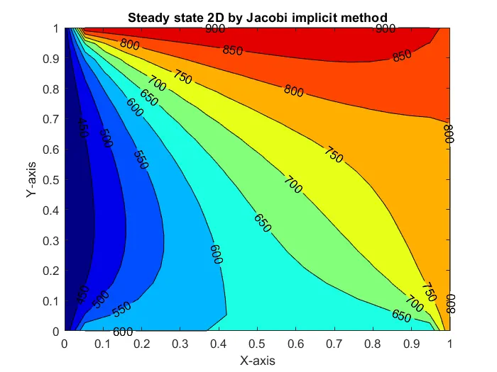
These are converging at below iterations
1) Jacobi = 826
2) GS = 442
3) SOR= 368
Conclusion: The time required to find out solution for temperature is longest for Jacobi method ,following second longest for GS and then Fastest converging scheme is SOR.
3) Explicit scheme- Transient state
The governing equation is,
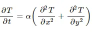
where  is time domain of temperature and
 is space domain .
Discretization of above equation is below


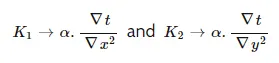 , where K1 and K2 are called CFL number.
Now, below is the program for the same,
%% Explicit method

% Unsteady, 2D, heat conduction solving in explicit way.

clear all
close all
clc

% Inputs
alpha = 1.4; % thermal diffusivity
nx = 10; % no of nodes on x axis
ny = 10;  % no of nodes on y axis
nt = 400; % no. of time steps

%Length of the domain
x = linspace(0,1,nx);
y = linspace(0,1,ny);

[xx yy] = meshgrid(x,y); % creating points in 2D

%Defining temperature at all grid points
T = 300*ones(nx, ny);

%Boundary conditions
T(1,:) = 600;
T(end,:) = 900;
T(:,1) = 400;
T(:,end) = 800;

nt= 1400; % Time steps
dt = 0.001;  % Time interval

dx = x(2)-x(1);
dy = y(2)-y(1);

% CFL values
k1 = alpha*(dt/ (dx^2));
k2 = alpha*(dt/ (dy^2));

% CFL in explicit should be less than or equal to 0.5 (k1+k2)(Diffusion
% problem)

T_old = T;

explicit_it = 1;
% time loop

tolerance = 1e-4;
tic

for k = 1: nt

    error = 9e9
while(error >tolerance)

  % space loop
for i= 2: nx -1
    for j= 2: ny-1

        term1(i,j) = (1-2*k1-2*k2)* T_old(i,j);
        term2(i,j) = k1*(T_old(i-1,j) + T_old(i+1,j));
        term3(i,j) = k2*(T_old(i,j+1) + T_old(i,j-1));

        T(i,j)= term1(i,j) + term2(i,j) + term3(i,j);

    end
end
error = max(max(abs(T-T_old)));
T_old = T ;
explicit_it = explicit_it +1;

end
iteration_time = toc

figure(1)
contourf(x,y,T)
colorbar
[a, b]= contourf(x,y,T);
clabel(a,b);
colormap(jet)
xlabel('X-axis')
ylabel('Y-axis')

title_text = sprintf('No. of iterations = %d iteration time = %d', explicit_it, iteration_time)
title(title_text)
pause(0.03)
end
Output:
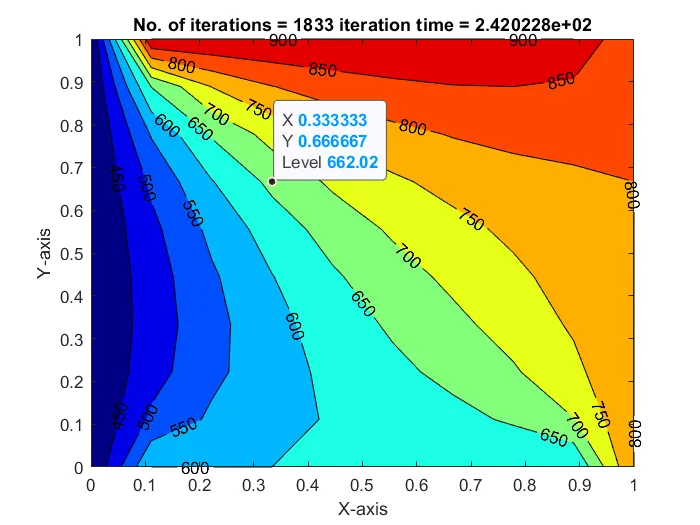
Explaination:
1) All input parameters are defined at the initial stage as x,y,dt,dx,dy. Length of x and y axes are 1m each.
2) After that, k1 and k2 are found out.After declaring all the inputs and constants the solution of equation will begin with convergence loop which runs until maximum value of temperature will reach upto tolerance value of 1e-4.
3) This process undergoes through time loop of 400 time steps.
4) Results are plotted. Number of iterations when solution converges comes out to be 1833 iterations.