Week 7 - Simulation of a 1D Super-sonic nozzle flow simulation using Macormack Method
Objective:
- To write code to solve the 1D supersonic nozzle flow equations using the Macormack Method by implementing both the conservative and non-conservative forms of the governing equations.
- Perform grid dependence test.
- To figure out the minimum number of cycles for which the simulation should be run in order of convergence.
- To compare the normalised mass flow rate between the conservative forms and non- conservative forms.
Non- Conservative form of governing equation:
Continuity equation:
`(dρ´)/(dt´)=-ρ´.(dV´)/(dx´)-ρ´.V´.d(logA´)/(dx´)-V´.(dρ´)/(dx´)`
Momentum equation:
`(dV´)/(dt´)=-V´(dV´)/(dx´)-(1/ϒ)((dT´)/(dx´)+(T´)/(ρ´) (dρ´)/(dx´))`
Energy equation:
`(dT´)/(dt´)=-V´(dT´)/(dx´)-(ϒ-1)T´((dV´)/(dx´)+V´d(logA´)/(dx´))`
All the variables are in non-dimensional form.
ρ = 1-0.3146x`d(ρ´A´V´)/(dt´)+d(ρ´A´V´^2+(1/ϒ)ρ´A´)/(dx´)=(1/ϒ)ρ´(dA´)/(dx´)`
t = 1-02314x
A= 1+2.2(x-1.5)2
Boundary conditions:
Inlet:
v (1) =2*v (2)-v (3)
Outlet:
v(n)=2*v(n-1)-v(n-2)
rho(n)=2*rho(n-1)-rho(n-2)
t(n)=2*t(n-1)-t(n-2)
Conservative form of governing equation:
`d(ρ´A´)/(dt´)=-d(ρ´A´V´)/(dx´)`
Momentum equation:
`d(ρ´A´V´)/(dt´)+d(ρ´A´V´^2+(1/ϒ)ρ´A´)/(dx´)=(1/ϒ)ρ´(dA´)/(dx´)`
Energy equation:
`d(ρ´(T´1/(ϒ-1)+(ϒ/2)V´^2 )A´)/(dt´)= -d(ρ´(T´1/(ϒ-1)+(ϒ/2)V´^2 )V´A´+ρ´A´V´)/(dx´)`
The above equation can be simplified in to the following equations;
U₁ = ρ´ A´
U₂ = ρ´A´V´
`U₃ = ρ´(T´1/(ϒ-1)+ϒ/2 V´^2 )A´`
F1 = ρ´A´V´
`F2 =ρ´A´V´^2+1/ϒ ρ´A´`
`F3 = ρ´(T´1/(ϒ-1)+ϒ/(2 ) V´^2 )V´A´+ρ´A´V´`
`J2 = 1/ϒ ρ´(dA´)/(dx´)`
Where U1, U2, U3 are called the solution vector, F1, F2, F3 are flux vectors and J2 is called source item.
Substituting the above term in governing equation we get:
`(dU₁)/(dt´)=-(dF₁)/(dx´)`
`(dU₂)/(dt´)=J^2-(dF₂)/(dx´)`
`(dU₃)/(dt´)=-(dF₃)/(dx´)`
Initial conditions;
`ρ=1-0.3146x`
`t=1-0.2314x`
`A=1+2.3(x-1.5)²`
Boundary conditions:
Inlet:
v (1) = 2*v (2)-v (3)
Outlet:
v(n)=2*v(n-1)-v(n-2)
rho(n)=2*rho(n-1)-rho(n-2)
t(n)=2*t(n-1)-t(n-2)
Discretization using Macormack Method
Steps in Macormack Method
Predictor step
`df/(dtₚ)`
Solution update: 󠄀
`f^'=fold +(df/(dtₚ)).Δt`
Corrector step:
`(df´)/〖dt〗_c`
Calculating average:
`(df/dt)_avg=0.5(df/(dtₚ)+(df´)/〖dt〗_c )`
Final solution update:
`f=f_old+(df/dt)_avg .Δt`
NON CONSERVATIVE
function [m_nc]=supersonic_nozzle_non_conservative(n,tol)
tic
%grid
x=linspace(0,3,n);

dx=x(2)-x(1);
gamma=1.4;
%specify throat
throat=(n+1)/2;
 m_analytical=0.579*ones(1,n);

C=0.5;
%initial profiles
rho=1-0.3146*x;
t=1-0.2314*x;   %Temperature
v=(0.1+1.09*x).*t.^0.5;
rho_old=rho;
v_old=v;
t_old=t;
%area
a=1+2.2*(x-1.5).^2;
%time steps
nt=1400;
nt_step=linspace(1,nt,nt);
for p=1:n
    dt_a(p)=C*dx/(t(p)^0.5+v(p));
end
dt=min(dt_a);
%outer time loop
iter=1;
error_rho=9e9;
error_v=9e9;
error_t=9e9;
for k=1:nt
     rho_old=rho;
     v_old=v;
     t_old=t;


    %predictor method
    for j=2:n-1
        dvdx=(v(j+1)-v(j))/dx;
        drhodx=(rho(j+1)-rho(j))/dx;
        dtdx=(t(j+1)-t(j))/dx;
        dlogadx=(log(a(j+1))-log(a(j)))/dx;

        %continuity equation
        drhodt_p(j)=-rho(j)*dvdx-rho(j)*v(j)*dlogadx-v(j)*drhodx;

        %momentum equation
        dvdt_p(j)=-v(j)*dvdx-(1/gamma)*(dtdx+(t(j)/rho(j))*drhodx);

        %energy equation
        dtdt_p(j)=-v(j)*dtdx-(gamma-1)*t(j)*(dvdx+v(j)*dlogadx);

        %solution update
        rho(j)=rho(j)+drhodt_p(j)*dt;
        v(j)=v(j)+dvdt_p(j)*dt;
        t(j)=t(j)+dtdt_p(j)*dt;
    end
    %corrector method
    for j=2:n-1
        dvdx=(v(j)-v(j-1))/dx;
        drhodx=(rho(j)-rho(j-1))/dx;
        dtdx=(t(j)-t(j-1))/dx;
        dlogadx=(log(a(j))-log(a(j-1)))/dx;

        %continuity equation
        drhodt_c(j)=-rho(j)*dvdx-rho(j)*v(j)*dlogadx-v(j)*drhodx;

        %momentum equation
        dvdt_c(j)=-v(j)*dvdx-(1/gamma)*(dtdx+(t(j)/rho(j))*drhodx);

        %energy equation
        dtdt_c(j)=-v(j)*dtdx-(gamma-1)*t(j)*(dvdx+v(j)*dlogadx);

    end
 %compute avg time derivative
 drhodt=0.5*(drhodt_p+drhodt_c);
 dvdt=0.5*(dvdt_p+dvdt_c);
 dtdt=0.5*(dtdt_p+dtdt_c);

 %final solution update
 for i=2:n-1
 rho(i)=rho_old(i)+drhodt(i)*dt;
 v(i)=v_old(i)+dvdt(i)*dt;
 t(i)=t_old(i)+dtdt(i)*dt;
 end
 M=v./t.^0.5;
 m_nc=rho.*a.*v;
  m_nct(k,:)=rho.*a.*v;
   error_rho=max(abs(rho-rho_old));
  error_v=max(abs(v-v_old));
  error_t=max(abs(t-t_old));
  if (error_rho>tol && error_v>tol && error_t>tol)
      iter=iter+1;

  end
 %apply boundary conditions
 %inlet
 v(1)=2*v(2)-v(3);
 %outlet
  v(n)=2*v(n-1)-v(n-2);
   rho(n)=2*rho(n-1)-rho(n-2);
    t(n)=2*t(n-1)-t(n-2);


end
rho_throat=rho(throat);
  v_throat=v(throat);
   t_throat=t(throat);
    M_throat=M(throat);
 figure(1)
    subplot(4,1,2)
    plot(x,rho,'linewidth',2)

    xlabel('nozzle length')
    ylabel('density ratio')
    subplot(4,1,3)
    plot(x,v,'r','linewidth',2)

    xlabel('nozzle length')
    ylabel('velocity ratio')
    subplot(4,1,4)
    plot(x,t,'g','linewidth',2)

    xlabel('nozzle length')
    ylabel('Temperature ratio')
    subplot(4,1,1)
    plot(x,M,'m','linewidth',2)
    title(sprintf('No of timestep=%d, no of iteration to steady state=%d',k,iter))
    xlabel('nozzle length')
    ylabel('Mach number')
%     suptitle('Non-conservative form')


     figure(3)
     plot(x,m_nct(50,:),x,m_nct(100,:),x,m_nct(200,:),x,m_nct(300,:),x,m_nct(500,:),'o',x,m_analytical,'linewidth',2)
     xlabel('non-dimensional distance x')
     ylabel('non-dimentional mass flow rate')
     title('variation of mass flow rate(non-conservative)')
     legend('50dt','100dt','200dt','300dt','700dt','analytical')
    time_nc=toc;
    fprintf('time of simlulation for nonconservative=%gsn',time_nc);
end
CONSERVATIVE
function [m_c]=supersonic_nozzl_conservative(n,tol)
tic
%grid
x=linspace(0,3,n);
dx=x(2)-x(1);
gamma=1.4;
throat=(n+1)/2;
m_analytical=0.579*ones(1,n);
%initial profiles
for q=1:n
    if ((x(q)>=0) && (x(q)<=0.5))
    rho(q)=1;
    t(q)=1;
    elseif ((x(q)<1.5) && (x(q)>0.5))
        rho(q)=1-0.366*(x(q)-0.5);
        t(q)=1-0.167*(x(q)-0.5);
    elseif ((x(q)>=1.5) && (x(q)<=3.5))
        rho(q)=0.634-0.3879*(x(q)-1.5);
        t(q)=0.833-0.03507*(x(q)-1.5);
    end
end
%area
a=1+2.2*(x-1.5).^2;
 v=0.59./(rho.*a);
U1=rho.*a;
U2=rho.*a.*v;
U3=rho.*(t./(gamma-1)+(gamma/2)*v.^2).*a;
%time steps
nt=1400;
nt_step=linspace(1,nt,nt);
C=0.5;
for p=1:n
    dt_a(p)=C*dx/(t(p)^0.5+v(p));
end
    dt=min(dt_a);
%outer time loop
iter=1;
 error_rho=9e9;
 error_v=9e9;
 error_t=9e9;
for k=1:nt
     U1_old=U1;
     U2_old=U2;
     U3_old=U3;
     rho_old=U1_old./a;
    v_old=U2_old./U1_old;
    t_old=(gamma-1)*((U3_old./U1_old)-(gamma/2)*v_old.^2);
      F1=U2;
     F2=(U2.^2)./U1+((gamma-1)/gamma)*(U3-(gamma/2)*(U2.^2)./U1);
     F3=(gamma*U2.*U3)./U1-((gamma*(gamma-1)/2)*(U2.^3)./U1.^2);


    %predictor method
    for j=2:n-1
       J2(j)=(1/gamma)*rho(j)*t(j)*(a(j+1)-a(j))/dx;

        %continuity equation
        dU1dt_p(j)=-(F1(j+1)-F1(j))/dx;

        %momentum equation
        dU2dt_p(j)=J2(j)-(F2(j+1)-F2(j))/dx;

        %energy equation
        dU3dt_p(j)=-(F3(j+1)-F3(j))/dx;


        %solution update
        U1(j)=U1(j)+dU1dt_p(j)*dt;
        U2(j)=U2(j)+dU2dt_p(j)*dt;
        U3(j)=U3(j)+dU3dt_p(j)*dt;
    end
    rho=U1./a;
    v=U2./U1;
    t=(gamma-1)*((U3./U1)-(gamma/2)*v.^2);
    F1=U2;
     F2=(U2.^2)./U1+((gamma-1)/gamma)*(U3-(gamma/2)*(U2.^2)./U1);
     F3=(gamma*U2.*U3)./U1-((gamma*(gamma-1)/2)*((U2.^3)./(U1.^2)));

    %corrector method
    for j=2:n-1
         J2(j)=(1/gamma)*rho(j)*t(j)*(a(j)-a(j-1))/dx;
         %continuity equation
        dU1dt_c(j)=-(F1(j)-F1(j-1))/dx;

        %momentum equation
        dU2dt_c(j)=J2(j)-(F2(j)-F2(j-1))/dx;

        %energy equation
        dU3dt_c(j)=-(F3(j)-F3(j-1))/dx;


    end
 %compute avg time derivative
 dU1dt=0.5*(dU1dt_p+dU1dt_c);
 dU2dt=0.5*(dU2dt_p+dU2dt_c);
 dU3dt=0.5*(dU3dt_p+dU3dt_c);

 %final solution update
 for i=2:n-1
 U1(i)=U1_old(i)+dU1dt(i)*dt;
 U2(i)=U2_old(i)+dU2dt(i)*dt;
 U3(i)=U3_old(i)+dU3dt(i)*dt;
 end

 %apply boundary conditions
 %inlet

U1(1)=rho(1).*a(1);
  U2(1)=2*U2(2)-U2(3);
   v(1)=U2(1)/(rho(1)*a(1));
U3(1)=U1(1)*(t(1)/(gamma-1)+(gamma/2)*v(1)^2);
 %outlet
  U2(n)=2*U2(n-1)-U2(n-2);
   U1(n)=2*U1(n-1)-U1(n-2);
    U3(n)=2*U3(n-1)-U3(n-2);
    %updating vlues
    rho=U1./a;
    v=U2./U1;
    t=(gamma-1)*((U3./U1)-(gamma/2)*v.^2);
    M=v./t.^0.5;
 m_c=rho.*a.*v;
 m_nc(k,:)=rho.*a.*v;

    error_rho=max(abs(rho-rho_old));
    error_v=max(abs(v-v_old));
 error_t=max(abs(t-t_old));
  if (error_rho>tol && error_v>tol && error_t>tol)
      iter=iter+1;
  end

end
rho_throat=rho(throat);
  v_throat=v(throat);
   t_throat=t(throat);
    M_throat=M(throat);
 figure(2)
   subplot(4,1,2)
    plot(x,rho,'linewidth',2)

    xlabel('nozzle length')
    ylabel('density ratio')
    subplot(4,1,3)
    plot(x,v,'r','linewidth',2)

    xlabel('nozzle length')
    ylabel('velocity ratio')
    subplot(4,1,4)
    plot(x,t,'g','linewidth',2)

    xlabel('nozzle length')
    ylabel('Temperature ratio')
    subplot(4,1,1)
    plot(x,M,'m','linewidth',2)
    title(sprintf('No of timestep=%d ,no of iteration to steady state=%d',k,iter))
    xlabel('nozzle length')
    ylabel('Mach number')
%     suptitle('Conservative form')


     figure(4)
     plot(x,m_nc(50,:),x,m_nc(100,:),x,m_nc(200,:),x,m_nc(300,:),x,m_nc(700,:),'o',x,m_analytical,'linewidth',2)
     xlabel('non-dimensional distance x')
     ylabel('non-dimentional mass flow rate')
     title('variation of mass flow rate(conservative)')
     legend('50dt','100dt','200dt','300dt','700dt','analytical')
      time_c=toc;
      fprintf('time of simlulation for conservative=%gsn',time_c);
end
MAIN PROGRAM
close all;
clear all;
clc;
n=31;
x=linspace(0,3,n);
tol=1e-4;
m_analytical=0.579*ones(1,n);
[m_nc]=supersonic_nozzle_non_conservative(n,tol);
[m_c]=supersonic_nozzl_conservative(n,tol);
    figure(5)
    plot(x,m_nc,'linewidth',2)
    hold on
    plot(x,m_c,'linewidth',2)
    hold on
     plot(x,m_analytical,'linewidth',2)
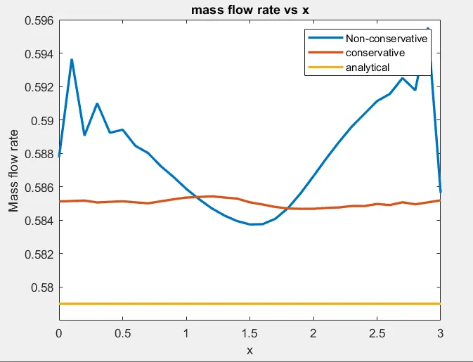
    title('mass flow rate vs x')
    xlabel('x')
    ylabel('Mass flow rate')
    legend('Non-conservative','conservative','analytical')
GRAPH
FIGURE 1
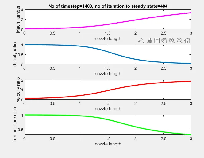
FIGURE 2
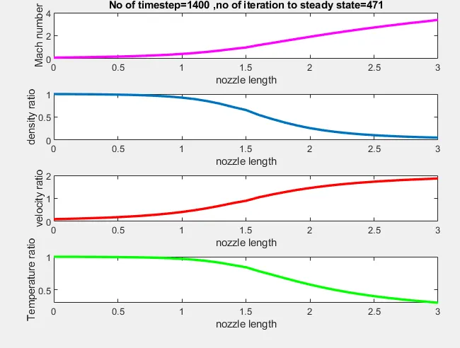
FIGURE 3
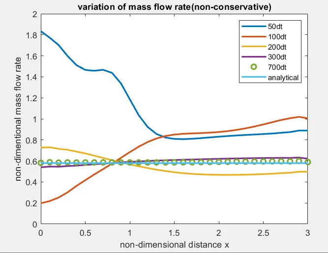
FIGURE 4
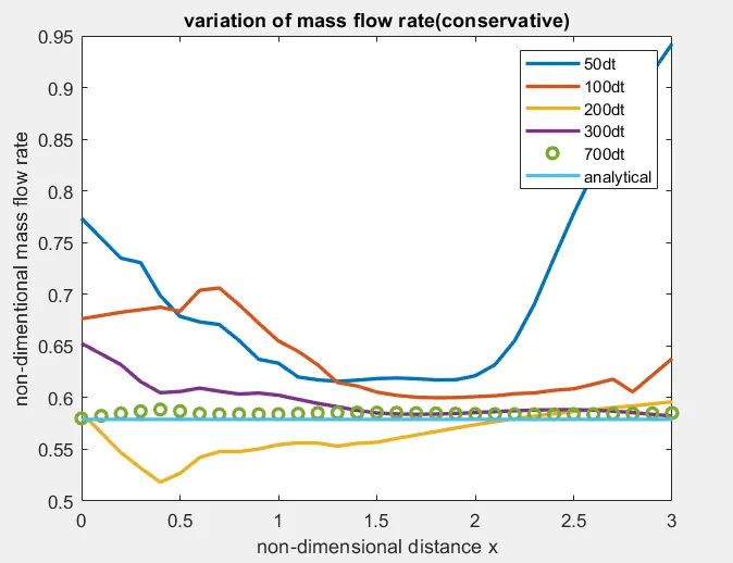
FIGURE 5