Week 3.5 - Deriving 4th order approximation of a 2nd order derivative using Taylor Table method

In this challenge a program was developed for calculation of 4^th order approximations of the second order derivative

For,

1. Central difference
2. Skewed right sided difference
3. Skewed left sided difference

1. Central difference:

The second order derivative can be written as:

`(∂^2 u)/(∂x^2 ) = "a.ƒ (i – 2) +b.ƒ (i– 1) +c.ƒ (i) +d.ƒ (i +1) +e.ƒ (i +2)"`

`ƒ´´(x) + Ox^2 = [a.ƒ(i –2)+b.ƒ(i – 1) +c.ƒ(i) +d.ƒ(i +1) +e.ƒ(i +2)]/Δx^2`

Solving the system of equation in MATLAB, we get the constants:

n3=[1,1,1,1,1;-2,-1,0,1,2;2,0.5,0,0.5,2;-8/6,-1/6,0,1/6,8/6;16/24,1/24,0,1/24,16/24];

m3=[0;0;1;0;0];

x3=inv(n3)*m3;

x3 =

   -0.0833
    1.3333
   -2.5000
    1.3333
   -0.0833

2. Skewed right sided difference:

The second order derivative can be written as:

`(∂^2 u)/(∂x^2 ) ="a.ƒ(i)+b.ƒ(i+1) +c.ƒ(i+2) +d.ƒ(i+3) +e.ƒ(i+4) +h.ƒ(i+5)"`

`ƒ´´(x) +Ox^4 = [a.ƒ(i)+b.ƒ(i+1) +c.ƒ(i+2) +d.ƒ(i+3) +e.ƒ(i+4) +h.ƒ(i+5)]/Δx^2`

n1=[1,1,1,1,1,1;0,1,2,3,4,5;0,0.5,2,4.5,8,12.5;0,1/6,8/6,27/6,64/6,125/6;0,1/24,16/24,81/24,256/24,625/24;0,1/120,32/120,243/120,1024/120,3125/120];

m1=[0;0;1;0;0;0];

x1=inv(n1)*m1;

x1 =

    3.7500
  -12.8333
   17.8333
  -13.0000
    5.0833
   -0.8333

3. Skewed left sided difference:

The second order derivative can be written as:

`(∂^2 u)/(∂x^2 ) = "a.ƒ (i – 5) +b.ƒ (i– 4) +c.ƒ (i – 3) +d.ƒ (i – 2) +e.ƒ (i –1) +h.ƒ(i)"`

`ƒ´´(x) + Ox^4 = [a.ƒ(i –5)+b.ƒ(i – 4) +c.ƒ(i –3) +d.ƒ(i –2) +e.ƒ(i –1) +h.ƒ(i)]/Δx^2`

n2=[1,1,1,1,1,1;-5,-4,-3,-2,-1,0;12.5,8,4.5,2,0.5,0;-125/6,-64/6,-27/6,-8/6,-1/6,0;625/24,256/24,81/24,16/24,1/24,0;-3125/120,-1024/120,-243/120,-32/120,-1/120,0];

m2=[0;0;1;0;0;0];

x2=inv(n2)*m2;

-0.8333
    5.0833
  -13.0000
   17.8333
  -12.8333
    3.7500

% function for central difference

function error_one=central_difference(x,dx)

a=-0.0833;b=1.3333;c=-2.5000;d=1.3333;e=-0.0833;

analytical_derivative=-2*exp(x)*sin(x);

calc_central=(a*exp(x-2*dx)*cos(x-2*dx)+b*exp(x-dx)*cos(x-dx)+c*exp(x)*cos(x)+d*exp(x+dx)*cos(x+dx)+e*exp(x+2*dx)*cos(x+2*dx))/(dx^2);

error_one=abs(analytical_derivative-calc_central);

end

% function for right difference

function error_two=right_sided_difference(x,dx)

a=3.7500;b=-12.8333;c=17.8333;d=-13.0000;e=5.0833;h=-0.8333;

analytical_derivative=-2*exp(x)*sin(x);

calc_right=(a*exp(x)*cos(x)+b*exp(x+dx)*cos(x+dx)+c*exp(x+2*dx)*cos(x+2*dx)+d*exp(x+3*dx)*cos(x+3*dx)+e*exp(x+4*dx)*cos(x+4*dx)+h*exp(x+5*dx)*cos(x+5*dx))/(dx^2);

error_two=abs(analytical_derivative-calc_right);

end

% function for left difference

function error_three=left_sided_difference(x,dx)

a=-0.8333333333;b=5.083333333;c=-13.0000;d=17.833333333;e=-12.8333333333;h=3.7500;

analytical_derivative=-2*exp(x)*sin(x);

calc_left=(a*exp(x-5*dx)*cos(x-5*dx)+b*exp(x-4*dx)*cos(x-4*dx)+c*exp(x-3*dx)*cos(x-3*dx)+d*exp(x-2*dx)*cos(x-2*dx)+e*exp(x-dx)*cos(x-dx)+h*exp(x)*cos(x))/(dx^2);

error_three=abs(analytical_derivative-calc_left);

end

MAIN PROGRAM

clear all;
close all;
clc;
x=pi;
dx=linspace(pi/4,pi/50,50);

for i=1:length(dx);
    
    error_one(i)=central_difference(x,dx(i));
    error_two(i)=right_sided_difference(x,dx(i));
    error_three(i)=left_sided_difference(x,dx(i));
    
end

 loglog(dx,error_one,'b');
 hold on
loglog(dx,error_two,'r');
 hold on
 plot(dx,error_three,'g');
 xlabel('dx');
ylabel('absolute error')
legend('central difference','right difference','left difference');

GRAPH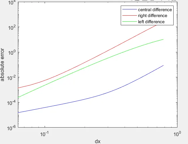

From the graph it is concluded that Central differencing scheme has less error

Skwed scheme is useful when information is from one side.