Week 7 - Simulation of a 1D Super-sonic nozzle flow simulation using Macormack Method
Objective:-
Solving the conservative and non-conservative forms of the governing equations through MacCormack method and comparing the results
Studying the variation of mass flow rate inside the nozzle at different time steps
Theory:-
A nozzle is a device designed to control the direction or characteristics of a fluid flow (especially to increase velocity) as it exits (or enters) an enclosed chamber or pipe.
A nozzle is often a pipe or tube of varying cross-sectional area, and it can be used to direct or modify the flow of a fluid. Nozzles are frequently used to control the rate of flow, speed, direction, mass, shape, and/or the pressure of the stream that emerges from them. In a nozzle, the velocity of fluid increases at the expense of its pressure energy.
A convergent-divergent nozzle is a device used to increase the velocity of a hot pressurized gas passing through it. It converts the enthalpy energy into kinetic energy.
In the field of CFD, MacCormack method is a prominent discretization scheme for obtaining numerical solution of a hyperbolic partial differential equations.
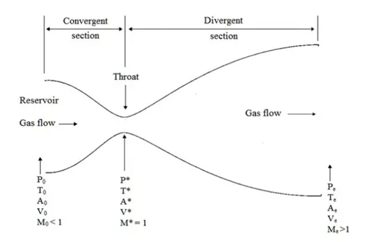
The area function for the CD nozzle is given as
`(A/A^*)^2 = 1 + 2.2*(x-1.5)^2` `0<=x<=3`
Where, `A^*` is the area at the throat of the nozzle and x is the distance along the length of the nozzle
The non-dimensionalized form of the variables required for this problem are,
`X^’ = x/L`
`V^’ = V/a_0`
`T^' = t/(L/a_0)`
`rho^’ = rho/rho_0`
`T^’ = T/T_0`
`p^’ = p/p_0`
`A^’ = A/A^*`
Governing equations:
- Non-conservative form
The non-conservative form of the governing equation which represent continuity, momentum and energy in terms of non-dimensionless variables
Continuity equation
`(delrho^’)/(delt^’) = -rho^’*(delV^’)/(delx^’) – rho^’*V^’*(del(lnA^’))/(delx^’) – V^’*(delrho^’)/(delx^’)`
Momentum equation
`(rhoV^’)/(delt^’) = -V^’*(delV^’)/(delx^’) – (1/gamma)*[(delT^’)/(delx^’) + (T^’/rho^’) * (delrho^’)/(delx^’)]`
Energy equation
`(delT^’)/(delt^’) = -V^’*(delT^’)/(delx^’) – (gamma – 1)*T^’*[(delV^’)/(delx^’) + V^’*(del(lnA^’))/(delx^’)]`
Initial Conditions
`rho^’ = 1-0.3146*x^’`
`T^’ = 1-0.2314*x^’`
`V^’ = (0.1+1.09*x^’)*sqrtT`
- Conservative form
The conservative form of governing equation which represents continuity, momentum and energy in non-dimensionalized form is given as
Continuity equation
`(del(rho^’*A^’))/(delt^’) + (del(rho^’*A^’*V^’))/(delx^’) = 0`
Momentum equation
`(del(rho^’*A^’*V^’))/(delt^’) + (del(rho^’*A^’*(V^’)^2 + (1/gamma)*rho^’*A^’))/(dx^’) = (1/gamma)*rho^’*(delA^’)/(delx^’)`
Energy equation
`(del(rho^’*((T^’)/(gamma-1) + gamma/2*(V^’)^2)*A^’))/(delt^’) + (del(rho^’*((T^’)/(gamma-1) + gamma/2*(V^’)^2)*V^’*A^’ + p^’*A^’*V^’))/(delx^’) = 0`
To solve the above equation, we will substitute the following terms, which include the solution vector U, the flux vector F and the source term J_2
`U_1 = rho^’*A^’`
`U_2 = rho^’*A^’*V^’`
`U_3 = rho^’*[(e^’)/(gamma-1) + (gamma/2)*(V^’)^2]*A^’`
`F_1 = rho^’*A^’*V^’ = U_2`
`F_2 = rho^’*A^’*(V^’)^2 + 1/gamma*P^’*A^’ = U_2/U_1 + (gamma-1)/gamma*(U_3 – gamma/2*(U_2^2)/U_1)`
`F_3 = rho^’*(e^’/(gamma-1) + gamma/2*(V^’)^2)*V^’*A^’ + P^’*A^’*V^’ = (gamma*U_2*U_3)/U_1 – gamma*(gamma-1)*2 * U_2^3/U_1^2`
`J_2 = 1/gamma*P^’*(delA^’)/(delx^’) = (gamma-1)/gamma * (U_3 – gamma/2*U_2^2/U_1)*(del(lnA^'))/(delx^’)`
Substituting these terms in the governing equations we get
`(delU_1)/(delt^’) = -(delF_1)/(delx^’)`
`(delU_2)/(delt^’) = -(delF_2)/(delx^’) + J_2`
`(delU_3)/(delt^’) = -(delF_3)/(delx^’)`
The flow variables can be calculated as
`rho^’ = U_1/A^’`
`V^’ = U_2/U_1`
`T^’ = e^’ = (gamma-1)*(U_3/U_1 – gamma/2*(V^’)^2)`
`P^’ = rho^’*T^’`
Initial conditions provided are as follows
`rho^’ = 1` for `0<=x^’<0.5`
`T^’ = 1`
`rho^’ = 1 – 0.366*(x^’-0.5)` for `0.5<=x^’<1.5`
`T^’ = 1 – 0.167*(x^’-0.5)`
`rho^’ = 0.634 – 0.3879*(x^’-1.5)` for `1.5<=x^’<=3.5`
`T^’ = 0.833 – 0.3507*(x^’-1.5)`
`V^’ = U_2/(rho^’*A^’)`
MacCormack method
The MacCormack numerical scheme is a common method to solve the flow equations. It basically consists of four steps
- Predictor step
- Intermediate solution update
- Corrector step
- Final solution update
In the predictor step, the spatial derivative are calculated using the forward difference scheme. This time derivative from the governing equations obtained is recorded as (delu/delt)_p. Consider, the continuity equation for the non-conservative form. From the predictor step, we obtain,
`((delrho_i)/(delt))_p = -rho_i^’[(V_(i+1)^’ – V_i^’)/Deltax^’] – rho_i^’*V_i^’*[(ln(A_(i+1)^’)-ln(A_i^’))/(Deltax^’)] – V_i^’*[(rho_(i+1)^’ – rho_i^’)/(Deltax^’)]`
During the intermediate solution update, the variable is updated based on the time derivative obtained from the predictor step
`(rho_i^(t+Deltat))_p = rho_i^’ + ((delrho_i^’)/(delt^’))_p *Deltat`
Using the updated values, the governing equations are solved again using the back differencing in space in the corrector step. The time derivative obtained during the corrector step is stored as ((delu)/(delt))_c
`((delrho_i)/(delt))_p = -rho_(i,p)^’[(V_(i,p)^’ – V_((i-1),p)^’)/(Deltax^’)] – rho_(i,p)^’*V_(i,p)^’*[(ln(A_(i,p)^’)-ln(A_((i-1),p)^’))/(Deltax^’)] – V_(i,p)^’*[(rho_(i,p)^’ – rho_((i-1),p)^’)/(Deltax^’)]`
For the final solution update, we use the average of the time-derivatives obtained using the predictor and the corrector steps. Since we are using forward difference in predictor step and backward difference in corrector step, the average of the time-derivative for the final update, the overall scheme becomes a second order numerical scheme.
`((delrho)/(delt))_(avg) = ½ * [((delrho)/(delt))_p + ((delrho)/(delt))_c]`
`rho_i^(t+Deltat) = rho_i^t + ((delrho)/(delt))_(avg)`
Matlab Program
n = 31
x = linspace(0,3,n)
dx = x(2)-x(1)
rho = 1 - (0.3146*x)
T = 1 - (0.2314*x)
V = (0.1 + (1.09*x)).*(T.^0.5)
A = 1 + (2.2.*(x-1.5).^2)
gamma = 1.4
C = 0.5

nt = 2000
dt = 0.01

[rho1,T1,V1,M1,m1,rho_t1,V_t1,T_t1,M1_t,residual1,p1,p1_t] = conservative(n,x,dx,nt,rho,V,T,A,gamma,C);
[rho2,T2,V2,M2,m2,rho_t2,V_t2,T_t2,M2_t,residual2,p2,p2_t] = non_conservative(n,x,dx,nt,rho,V,T,A,gamma,C)


 figure(1)
 subplot(4,1,1)
 plot(x,M1)
 ylabel('Mach number')
 title('Conservative form')
 subplot(4,1,2)
 plot(x,p1)
 ylabel('pressure ratio')
 subplot(4,1,3)
 plot(x,rho1)
 ylabel('density ratio')
 subplot(4,1,4)
 plot(x,T1)
 ylabel('temperature ratio')


 figure(2)
 subplot(4,1,1)
 plot(x,M2)
 ylabel('Mach number')
 title('Non-Conservative form')
 subplot(4,1,2)
 plot(x,p2)
 ylabel('pressure ratio')
 subplot(4,1,3)
 plot(x,rho2)
 ylabel('density ratio')
 subplot(4,1,4)
 plot(x,T2)
 ylabel('temperature ratio')


 figure(3)
 subplot(4,1,1)
 plot(1:nt,M1_t)
 ylabel('Mach number at throat')
 title('Conservative form')
 subplot(4,1,2)
 plot(1:nt,rho_t1)
 ylabel('Density at throat')
 subplot(4,1,3)
 plot(1:nt,p1_t)
 ylabel('pressure ratio at throat')
 subplot(4,1,4)
 plot(1:nt,T_t1)
 ylabel('Temperature ratio at throat')


 figure(4)
 subplot(4,1,1)
 plot(1:nt,M2_t)
 ylabel('Mach number at throat')
 title('Non-Conservative form')
 subplot(4,1,2)
 plot(1:nt,rho_t2)
 ylabel('Density at throat')
 subplot(4,1,3)
 plot(1:nt,p2_t)
 ylabel('pressure ratio at throat')
 subplot(4,1,4)
 plot(1:nt,T_t2)
 ylabel('Temperature ratio at throat')


 figure(5)
subplot(2,1,1)
plot(1:nt,residual1)
subplot(2,1,2)
plot(1:nt,residual2)

figure(6)
plot(x,m1(50,:))
hold on
plot(x,m1(100,:))
plot(x,m1(150,:))
plot(x,m1(200,:))
plot(x,m1(700,:))
xlabel('X/L')
ylabel('rhoAV/rho_0A_0V_0')
legend('t=50/t','t=100/t','t=150/t','t=200/t','t=700/t')
title('Variation of non dimensional mass flow rate (Conservative form)')

figure(7)
plot(x,m2(50,:))
hold on
plot(x,m2(100,:))
plot(x,m2(150,:))
plot(x,m2(200,:))
plot(x,m2(700,:))
xlabel('X/L')
ylabel('rhoAV/rho_0A_0V_0')
legend('t=50/t','t=100/t','t=150/t','t=200/t','t=700/t')
title('Variation of non dimensional mass flow rate (Non Conservative form)')

figure(8)
plot(x,m1(end,:))
hold on
plot(x,m2(end,:))
xlabel('X/L')
ylabel('rhoAV/rho_0A_0V_0')
legend('Conservative','Non-Conservative')
Function program for conservative and non-conservative
function [rho1,T1,V1,M1,m1,rho_t1,V_t1,T_t1,M1_t,residual1,p1,p1_t] = conservative(n,x,dx,nt,rho,V,T,A,gamma,C)

%Initial conditions
rho_0 = zeros(1,length(x));
T_0 = rho_0;
V_0 = rho_0;

for e = 1:length(x)
    if x(e)>=0 && x(e)< 0.5
        rho_0(e) = 1
        T_0(e) = 1
    elseif x(e)>=0.5 && x(e)<1.5
        rho_0(e) = 1 - (0.366*(x(e)-0.5))
        T_0(e) = 1 - (0.167*(x(e)-0.5))
    elseif x(e)>=1.5 && x(e)<=3.5
        rho_0(e) = 0.634 - (0.3879*(x(e)-1.5))
        T_0(e) = 0.833 - (0.3507*(x(e)-1.5))
    end
    V_0(e) = 0.59/(rho_0(e)*A(e))
end

rho1 = rho_0
T1 = T_0
V1 = V_0
throat = find(A==1)

m1 = zeros(nt,length(x))

rho_t1 = zeros(1,nt)
T_t1 = rho_t1
V_t1 = rho_t1
p1_t = V_t1
M1_t = V_t1
residual1 = zeros(nt,3)

U1 = rho1.*A
U2 = rho1.*A.*V1
U3 = rho1.*((T1./(gamma-1)) + (gamma/2).*(V1.^2)).*A

for g = 1:nt
    U1_old = U1;
    U2_old = U2;
    U3_old = U3;

    for o = 1:n
        dt_x(o) = (C*dx)/((T1(o)^0.5) + V1(o));
    end

    dt = min(dt_x)

    F1 = U2;
    F2 = ((U2.^2)./U1) + ((gamma-1)/gamma).*(U3 - (gamma/2).*((U2.^2)./U1));
    F3 = ((gamma.*U2.*U3)./U1) - (((gamma*(gamma-1))/2).*((U2.^3)./(U1.^2)));

    %Predictor step
    for e = 2:length(x)-1
        dF1dx_p = (F1(e+1) - F1(e))/dx;
        dF2dx_p = (F2(e+1) - F2(e))/dx;
        dF3dx_p = (F3(e+1) - F3(e))/dx;
        dAdx_p = ((A(e+1)-A(e))./dx);
        J = (1/gamma).*rho1(e).*T1(e).*(dAdx_p);


        dU1dt_p(e) = -(dF1dx_p);
        dU2dt_p(e) = -(dF2dx_p)+J;
        dU3dt_p(e) = -(dF3dx_p);

        %Update
        U1(e) = U1(e) + (dU1dt_p(e)*dt);
        U2(e) = U2(e) + (dU2dt_p(e)*dt);
        U3(e) = U3(e) + (dU3dt_p(e)*dt);
    end


    rho1 = U1./A;
    V1 = U2./U1;
    T1 = (gamma-1).*((U3./U1)-((gamma/2).*(V1.^2)));

    F1 = U2;
    F2 = ((U2.^2)./U1) + ((gamma-1)/gamma).*(U3 - (gamma/2).*((U2.^2)./U1));
    F3 = ((gamma.*U2.*U3)./U1) - (((gamma*(gamma-1))/2).*((U2.^3)./(U1.^2)));


    %Corrector step
    for j = 2:length(x)-1;
        dF1dx_c(j) = (F1(j) - F1(j-1))/dx;
        dF2dx_c(j) = (F2(j) - F2(j-1))/dx;
        dF3dx_c(j) = (F3(j) - F3(j-1))/dx;
        dAdx_p = ((A(j)-A(j-1))./dx);
        J = (1/gamma).*rho1(j).*T1(j).*(dAdx_p);

        dU1dt_c(j) = -(dF1dx_c(j));
        dU2dt_c(j) = -(dF2dx_c(j))+J;
        dU3dt_c(j) = -(dF3dx_c(j));
    end


    %Average step
    dU1dt_avg = 0.5*(dU1dt_p + dU1dt_c);
    dU2dt_avg = 0.5*(dU2dt_p + dU2dt_c);
    dU3dt_avg = 0.5*(dU3dt_p + dU3dt_c);

    residual1(g,1) = max(abs(dU1dt_avg));
    residual1(g,2) = max(abs(dU2dt_avg));
    residual1(g,3) = max(abs(dU3dt_avg));

    for k = 2:length(x)-1
        U1(k) = U1_old(k) + ((dU1dt_avg(k))*dt);
        U2(k) = U2_old(k) + ((dU2dt_avg(k))*dt);
        U3(k) = U3_old(k) + ((dU3dt_avg(k))*dt);
    end


    %Boundary conditions

    %Inlet conditions
    U1(1) = rho1(1)*A(1);
    U2(1) = (2*U2(2))-U2(3);
    V(1) = U2(1)/U1(1);
    U3(1) = U1(1)*((T1(1)/(gamma-1)) + ((gamma/2)*(V1(1))^2));

    %outlet conditions
    U1(end) = (2*U1(end-1))-U1(end-2);
    U2(end) = (2*U2(end-1))-U2(end-2);
    U3(end) = (2*U3(end-1))-U3(end-2);

    rho1 = U1./A;
    V1 = U2./U1;
    T1 = (gamma-1)*((U3./U1)-((gamma/2)*(V1.^2)));
    p1 = rho1.*T1;

    %Mach number
    for q = 1:n
        M1(q) = V1(q)./(T1(q).^0.5);
    end

    %Mass Flow Rate
    m1(g,:) = rho1.*A.*V1;

    %Parameters at the Throat

    rho_t1(g) = rho1(throat);
    V_t1(g) = V1(throat);
    T_t1(g) = T1(throat);
    M1_t(g) = M1(throat);
    p1_t(g) = p1(throat);

end
plot(x,rho1)
hold on
plot(x,T1)
plot(x,V1)
end
function [rho2,T2,V2,M2,m2,rho_t2,V_t2,T_t2,M2_t,residual2,p2,p2_t] = non_conservative(n,x,dx,nt,rho,V,T,A,gamma,C)
%Initial conditions
rho2 = rho
V2 = V
T2 = T
rho_t2 = zeros(1,nt)
T_t2 = rho_t2
V_t2 = T_t2
p2_t = T_t2
M2_t = T_t2
m2 = zeros(nt,length(x))
residual2 = zeros(nt,3)
throat = find(A==1)
for i = 1:nt
rho_old = rho2
V_old = V2
T_old = T2
for o = 1:n
dt_x(o) = (C*dx)/((T2(o)^0.5) + V2(o))
end
dt = min(dt_x);
for j = 2:n-1
%predictor step
dVdx = (V2(j+1)-V2(j))/dx;
drhodx = (rho2(j+1)-rho2(j))/dx;
dTdx = (T2(j+1)-T2(j))/dx;
dlogdx = (log(A(j+1))-log(A(j)))/dx;
drhodt_p(j) = (-rho2(j).*(dVdx)) - (rho2(j).*V2(j).*dlogdx) - (V2(j).*drhodx);
dVdt_p(j) = (-V2(j).*dVdx) - (1/gamma).*(dTdx + ((T2(j)./rho2(j)).*(drhodx)));
dTdt_p(j) = (-V2(j).*dTdx) - (((gamma-1).*T2(j)).*(dVdx + (V2(j).*dlogdx)));
rho_p2(j) = rho2(j) + (drhodt_p(j).*dt);
V_p2(j) = V2(j) + (dVdt_p(j).*dt);
T_p2(j) = T2(j) + (dTdt_p(j).*dt);
end
rho_p2(1) = rho2(1)
V_p2(1) = V2(1)
T_p2(1) = T2(1)
%Corrector step
for j = 2:n-1
%predictor step
dVdx = (V_p2(j)-V_p2(j-1))/dx;
drhodx = (rho_p2(j)-rho_p2(j-1))/dx;
dTdx = (T_p2(j)-T_p2(j-1))/dx;
dlogdx = (log(A(j))-log(A(j-1)))/dx;
drhodt_c(j) = (-rho2(j).*(dVdx)) - (rho2(j).*V2(j).*dlogdx) - (V2(j).*drhodx);
dVdt_c(j) = (-V2(j).*dVdx) - (1/gamma).*(dTdx + ((T2(j)./rho2(j)).*(drhodx)));
dTdt_c(j) = (-V2(j).*dTdx) - (((gamma-1).*T2(j)).*(dVdx + (V2(j).*dlogdx)));
end
%Average step
drhodt_avg = 0.5*(drhodt_p + drhodt_c);
dVdt_avg = 0.5*(dVdt_p + dVdt_c);
dTdt_avg = 0.5*(dTdt_p + dTdt_c);
residual2(i,1) = max(abs(drhodt_avg));
residual2(i,2) = max(abs(dVdt_avg));
residual2(i,3) = max(abs(dTdt_avg));
%solution update
for k = 2:n-1
rho2(k) = rho_old(k) + drhodt_avg(k)*dt;
V2(k) = V_old(k) + dVdt_avg(k)*dt;
T2(k) = T_old(k) + dTdt_avg(k)*dt;
end
%inlet condition
V2(1) = 2*V2(2)-V2(3);
T2(1) = 1;
rho2(1) = 1;
%outlet condition
V2(end) = 2*V2(end-1)-V2(end-2);
T2(end) = 2*T2(end-1)-T2(end-2);
rho2(end) = 2*rho2(end-1)-rho2(end-2);
M2 = V2./(T2.^0.5);
p2 = rho2.*T2;
m2(i,:) = rho2.*A.*V2;
%Parameters at the Throat
rho_t2(i) = rho2(throat);
V_t2(i) = V2(throat);
T_t2(i) = T2(throat);
M2_t(i) = M2(throat);
p2_t(i) = p2(throat);
end
plot(x,rho2)
hold on
plot(x,T2)
plot(x,V2)
endOutput
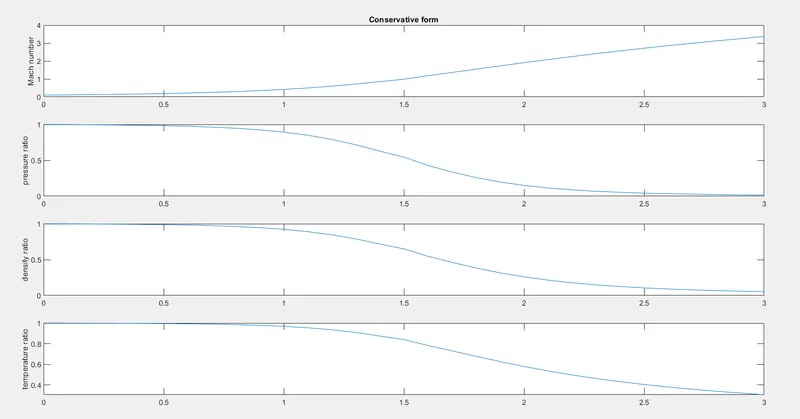
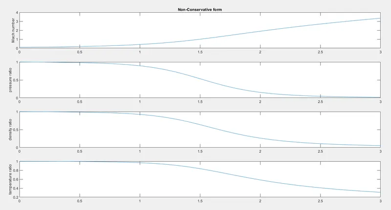
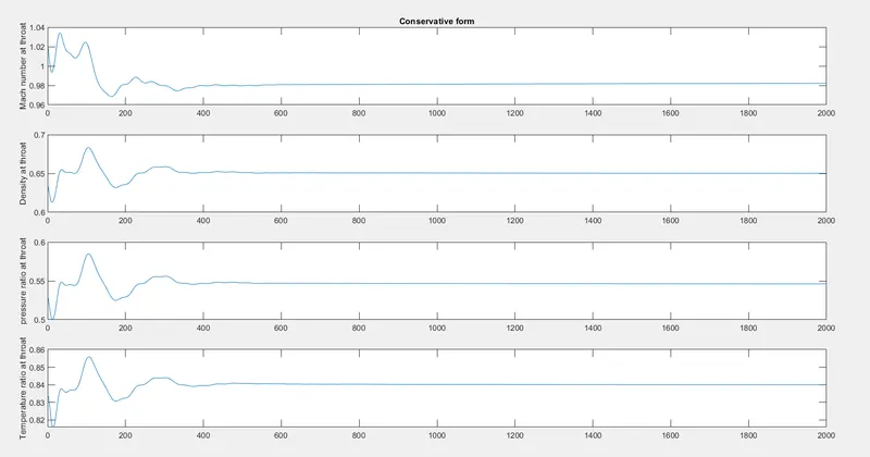
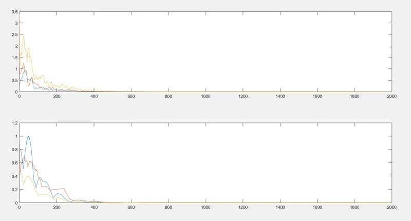
Residuals
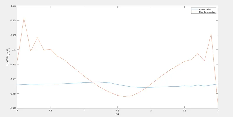
Mass flow rate
Conclusion
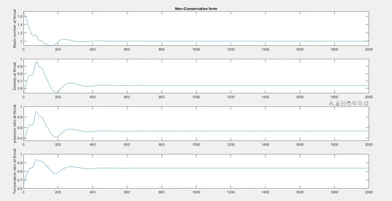
It can be observed that at smaller time-steps, the behavior of non-conservative form show unstable results. i.e oscillations are seen. As the time-step increases, it can be observed that there is no difference between the conservative and non-conservative method
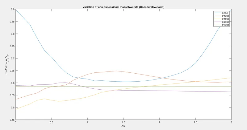
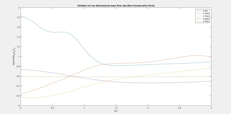
We can observe an appreciable difference in the mass flow rate as the time-step varies.
At the time step of `700Deltat`, the mass flow becomes constant. The conservative form produces an almost constant mass flow rate but the non-conservative approach gives a highly fluctuating mass flow rate
The non conservative provides more accuracy in case of primitive variables
Grid dependency Test
|
Density ratio |
Temperature ratio |
Pressure ratio |
M |
|
|
Exact analytical solution |
0.634 |
0.833 |
0.528 |
1 |
|
Conservative form (31 points) |
0.6524 |
0.841 |
0.5487 |
0.978 |
|
Non-conservative form (31 points) |
0.6387 |
0.8365 |
0.5342 |
0.9994 |
|
Conservative form (61 points) |
0.6391 |
0.8355 |
0.534 |
0.9979 |
|
Non-conservative form (61 points) |
0.6377 |
0.8354 |
0.5327 |
0.9998 |
The first row is the exact analytical results. The second and the third rows shows us the results for the conservative and non-conservative forms at n=31.
We can observe that the results from the non-conservative form are much closer to the exact values.
The fourth and the fifth rows shows us the results for the conservative and non-conservative forms at n=61.
Here we can observe that by increasing the number of grid points, the steady state numerical results are slightly close to the exact analytical values. We can observe that even after having 61 grid points for conservative form, still the results are not as close as the non-conservative form results with half as many grid points.
It can be finally concluded that the solution from both the forms are grid independent