Week 7 - Simulation of a 1D Super-sonic nozzle flow simulation using Macormack Method
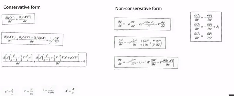
the governing equation for conservative and non conservative forms
The initial profile for a, rho, t and v as it is defined in CFD book by John Anderson.
x = linspace(0,3,n);
% calculate intial profiles
rho = 1-0.3146*x;
t = 1-0.2314*x; % t = temprature
v = (0.1+1.09*x).*t.^0.5;
% area
a = 1+2.2*(x-1.5).^2
- Non conservative governing equation of 1D supersonic nozzle flow:
The function talks n, nt, dt, gama, rho, t, v, a, and dx as inputs and massflow1, rho1, v1 and t1 as outputs. Then starting with for loop for total of time steps tn.
Inside this loop there is a second for loop for number of nodes “31” to calculate the predictor method for continuity, momentum, and energy equations.
for j = 2:n-1
dvdx = (v(j+1)-v(j))/dx;
drhodx = (rho(j+1)-rho(j))/dx;
dtdx = (t(j+1)-t(j))/dx;
dlogadx = (log(a(j+1))-log(a(j)))/dx;
% continuity equation
drhodt_p(j) = -rho(j)*dvdx - rho(j)*v(j)*dlogadx - v(j)*drhodx;
% momentum equation
dvdt_p(j) = -v(j)*dvdx - (1/gama)*(dtdx + (t(j)/rho(j))*drhodx);
% energy equation
dtdt_p(j) = -v(j)*dtdx - (gama -1)*t(j)*(dvdx + v(j)*dlogadx);
% solution update
rho(j) = rho(j) + drhodt_p(j)*dt;
v(j) = v(j) + dvdt_p(j)*dt;
t(j) = t(j) + dtdt_p(j)*dt;
end
Then the corrector method loop which calculate the correction equation for continuity, momentum, and energy equations.
for j = 2:n-1
dvdx = (v(j)-v(j-1))/dx;
drhodx = (rho(j)-rho(j-1))/dx;
dtdx = (t(j)-t(j-1))/dx;
dlogadx = (log(a(j))-log(a(j-1)))/dx;
% continuity equation
drhodt_c(j) = -rho(j)*dvdx - rho(j)*v(j)*dlogadx - v(j)*drhodx;
% momentum equation
dvdt_c(j) = -v(j)*dvdx - (1/gama)*(dtdx + (t(j)/rho(j))*drhodx);
% energy equation
dtdt_c(j) = -v(j)*dtdx - (gama -1)*t(j)*(dvdx + v(j)*dlogadx);
end
The average of predictor and corrector method will be calculated.
drhodt = 0.5*(drhodt_p + drhodt_c);
dvdt = 0.5*(dvdt_p + dvdt_c);
dtdt = 0.5*(dtdt_p + dtdt_c);
Then the new rho, v, and t values should be updated.
for i = 2:n-1
rho(i) = rho_old(i) + drhodt(i)*dt;
v(i) = v_old(i) + dvdt(i)*dt;
t(i) = t_old(i) + dtdt(i)*dt;
end
At the end, the boundary condition for inlet and outlet will be updated. % inlet
v(1) = 2*v(2) - v(3);
% outlet
v(n) = 2*v(n-1) - v(n-2);
rho(n) = 2*rho(n-1) - rho(n-2);
t(n) = 2*t(n-1) - t(n-2);
Then rho, v, t, and massflow for each time iteration will be save in function outputs.
rho1(k,:) = rho;
v1(k,:) = v;
t1(k,:) = t;
massflow1(k,:) = rho.*a.*v;
- Conservative method
The function has the same inputs and returns the same parameters.
To solve the conservative equation, I should define additional variables u1, u2, and u3.
u1 = rho.*a;
u2 = rho.*a.*v;
u3 = u1.*((t./(gama-1))+((gama/2).*(v.^2)));
Then inside a for loop for the number of time steps I defined the flux terms regarding new terms.
f1 = u2;
f2 = ((u2.^2)./u1)+(((gama-1)/gama)*(u3-((gama/2)*(u2.^2)./u1)));
f3 = ((gama*u2.*u3)./u1)-(gama*0.5*(gama-1)*(u2.^3)./(u1.^2));
After that inside a second for loop I calculated the predictor method for continuity, momentum, and energy equations. And updated the initial values as well. for j = 2:n-1
dadx = (a(j+1)-a(j))/dx;
j2 = (rho(j)*t(j)*dadx)/gama;
% continuity equation
du1dt_p(j) = -(f1(j+1)-f1(j))/dx;
% momentum equation
du2dt_p(j) = -(f2(j+1)-f2(j))/dx + j2;
% energy equation
du3dt_p(j) = -(f3(j+1)-f3(j))/dx;
% solution update
u1(j) = u1(j) + du1dt_p(j)*dt;
u2(j) = u2(j) + du2dt_p(j)*dt;
u3(j) = u3(j) + du3dt_p(j)*dt;
end
Then the prediction of the primitive.
rho = u1./a;
v = u2./u1;
t = (gama-1)*((u3./u1)-((gama/2)*(v.^2)));
f1 = u2;
f2 = ((u2.^2)./u1)+(((gama-1)/gama)*(u3-((gama/2)*(u2.^2)./u1)));
f3 = ((gama*u2.*u3)./u1)-(gama*0.5*(gama-1)*(u2.^3)./(u1.^2));
The second stage of maccormack method is the correction equation for continuity, momentum, and energy equations which will be written in separated for loop.
for j = 2:n-1
dadx = (a(j)-a(j-1))/dx;
j2 = (rho(j)*t(j)*dadx)/gama;
% continuity equation
du1dt_c(j) = -(f1(j)-f1(j-1))/dx;
% momentum equation
du2dt_c(j) = -(f2(j)-f2(j-1))/dx + j2;
% energy equation
du3dt_c(j) = -(f3(j)-f3(j-1))/dx;
end
Finally calculate the average and the final solution for current time derivative.
du1dt = 0.5*(du1dt_p + du1dt_c);
du2dt = 0.5*(du2dt_p + du2dt_c);
du3dt = 0.5*(du3dt_p + du3dt_c);
% final solution update
for i = 2:n-1
u1(i) = u1_old(i) + du1dt(i)*dt;
u2(i) = u2_old(i) + du2dt(i)*dt;
u3(i) = u3_old(i) + du3dt(i)*dt;
end
At the end applying the boundary conditions and return function outputs.
% inlet
u1(1) = rho(1)*a(1);
u2(1) = 2*u2(2) - u2(3);
v(1) = u2(1)/u1(1);
u3(1) = u1(1)*((t(1)/(gama-1))+((gama/2)*(v(1)^2)));
% outlet
u1(n) = 2*u1(n-1) - u1(n-2);
u2(n) = 2*u2(n-1) - u2(n-2);
u3(n) = 2*u3(n-1) - u3(n-2);
rho = u1./a;
v = u2./u1;
t = (gama-1)*((u3./u1)-((gama/2)*(v.^2)));
rho2(k,:) = rho;
v2(k,:) = v;
t2(k,:) = t;
massflow2(k,:) = rho.*a.*v;
Mach2(k,:) = v./(t.^0.5);
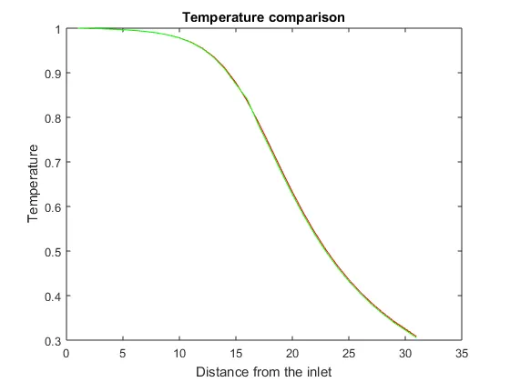
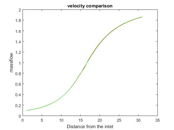
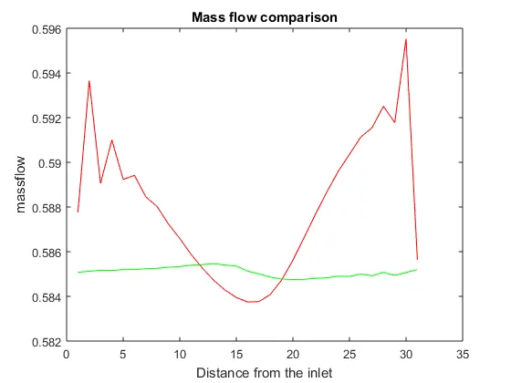
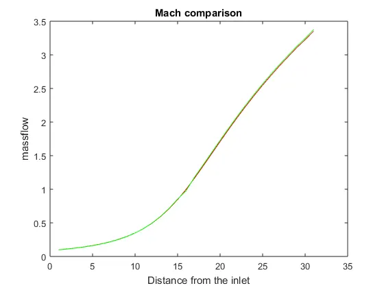
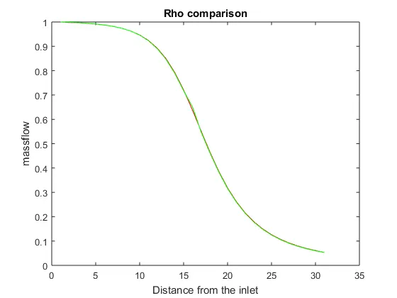
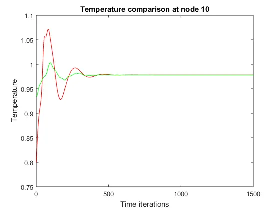
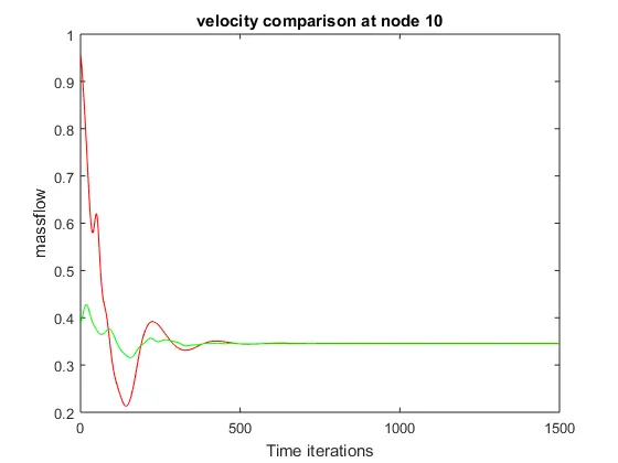
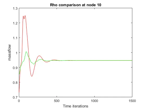
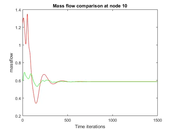
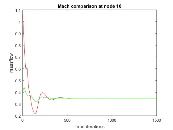
Conclusion:
The conversion time for both conservative and non-conservative forms are comparable about (tn=500).
There is not that big difference between the result of both forms.
The results also getting more accurate when the mesh is finer.
clear all
clear all
clc

% inputs
n = 31;
x = linspace(0,3,n);
dx = x(2)-x(1);
gama = 1.4;

% calculate intial profiles
rho = 1-0.3146*x;
t = 1-0.2314*x;  % t = temprature
v = (0.1+1.09*x).*t.^0.5;

% area
a = 1+2.2*(x-1.5).^2;

% Time steps
nt = 1500;
dt = 0.01;
dt_min1 = min(0.5.*(dx./((t.^0.5)+v)));
[Mach1,massflow1,rho1,v1,t1] = non_conservative_maccormack(n,nt,dt_min1,gama,rho,t,v,a,dx);

% Initial profiles
for i=1:n
    if (x(i)>0 && x(i)<=0.5)
    rho(i) = 1;
    t(i) = 1;
    elseif (x(i)>0.5 && x(i)<=1.5)
        rho(i) = 1-0.366*(x(i)-0.5);
        t(i) = 1-0.167*(x(i)-0.5);
    elseif (x(i)>1.5 && x(i)<=3.5)
        rho(i)= 0.634-0.3879*(x(i)-1.5);
        t(i) = 0.833-0.3507*(x(i)-1.5);
    end

end
v = 0.59./(rho.*a);
dt = 0.0001;
% minimum time step for stabilation
dt_min2 = min(0.5*(dx./((t.^0.5)+v)));
[Mach2,massflow2,rho2,v2,t2] = conservative_maccormack(n,nt,dt_min2,gama,rho,t,v,a,dx);

figure(1)
plot(t1(1500,:),'color','r');
hold on
plot(t2(1500,:),'color','g');
xlabel('Distance from the inlet');
ylabel('Temperature');
title('Temperature comparison ');

figure(2)
plot(v1(1500,:),'color','r');
hold on
plot(v2(1500,:),'color','g');
xlabel('Distance from the inlet');
ylabel('massflow');
title('velocity comparison');

figure(3)
plot(rho1(1500,:),'color','r');
hold on
plot(rho2(1500,:),'color','g');
xlabel('Distance from the inlet');
ylabel('massflow');
title('Rho comparison');

figure(4)
plot(Mach1(1500,:),'color','r');
hold on
plot(Mach2(1500,:),'color','g');
xlabel('Distance from the inlet');
ylabel('massflow');
title('Mach comparison');

figure(5)
plot(massflow1(1500,:),'color','r');
hold on
plot(massflow2(1500,:),'color','g');
xlabel('Distance from the inlet');
ylabel('massflow');
title('Mass flow comparison');


figure(6)
plot(t1(:,10),'color','r');
hold on
plot(t2(:,10),'color','g');
xlabel('Time iterations');
ylabel('Temperature');
title('Temperature comparison at node 10');

figure(7)
plot(v1(:,10),'color','r');
hold on
plot(v2(:,10),'color','g');
xlabel('Time iterations');
ylabel('massflow');
title('velocity comparison at node 10');

figure(8)
plot(rho1(:,10),'color','r');
hold on
plot(rho2(:,10),'color','g');
xlabel('Time iterations');
ylabel('massflow');
title('Rho comparison at node 10');

figure(9)
plot(Mach1(:,10),'color','r');
hold on
plot(Mach2(:,10),'color','g');
xlabel('Time iterations');
ylabel('massflow');
title('Mach comparison at node 10');

figure(10)
plot(massflow1(:,10),'color','r');
hold on
plot(massflow2(:,10),'color','g');
xlabel('Time iterations');
ylabel('massflow');
title('Mass flow comparison at node 10');
function [Mach2,massflow2, rho2,v2,t2] = conservative_maccormack(n,nt,dt,gama,rho,t,v,a,dx)

     % initial solution
    u1 = rho.*a;
    u2 = rho.*a.*v;
    u3 = u1.*((t./(gama-1))+((gama/2).*(v.^2)));

    % outer time loop
    for k = 1:nt

        %predictor method
        u1_old = u1;
        u2_old = u2;
        u3_old = u3;

        % flux terms regaeding new terms u1 u2 u3
        f1 = u2;
        f2 = ((u2.^2)./u1)+(((gama-1)/gama)*(u3-((gama/2)*(u2.^2)./u1)));
        f3 = ((gama*u2.*u3)./u1)-(gama*0.5*(gama-1)*(u2.^3)./(u1.^2));

        for j = 2:n-1

            dadx = (a(j+1)-a(j))/dx;
            j2 = (rho(j)*t(j)*dadx)/gama;
            % continuity equation
            du1dt_p(j) = -(f1(j+1)-f1(j))/dx;
            % momentum equation
            du2dt_p(j) = -(f2(j+1)-f2(j))/dx + j2;
            % energy equation
            du3dt_p(j) = -(f3(j+1)-f3(j))/dx;
            % solution update
            u1(j) = u1(j) + du1dt_p(j)*dt;
            u2(j) = u2(j) + du2dt_p(j)*dt;
            u3(j) = u3(j) + du3dt_p(j)*dt;

      end

        % prediction of the primitves
        rho = u1./a;
        v = u2./u1;
        t = (gama-1)*((u3./u1)-((gama/2)*(v.^2)));
        f1 = u2;
        f2 = ((u2.^2)./u1)+(((gama-1)/gama)*(u3-((gama/2)*(u2.^2)./u1)));
        f3 = ((gama*u2.*u3)./u1)-(gama*0.5*(gama-1)*(u2.^3)./(u1.^2));
        % corrector method
        for j = 2:n-1

            dadx = (a(j)-a(j-1))/dx;
            j2 = (rho(j)*t(j)*dadx)/gama;
            % continuity equation
            du1dt_c(j) = -(f1(j)-f1(j-1))/dx;
            % momentum equation
            du2dt_c(j) = -(f2(j)-f2(j-1))/dx + j2;
            % energy equation
            du3dt_c(j) = -(f3(j)-f3(j-1))/dx;

        end

        % cmpute the average time derivative
        du1dt = 0.5*(du1dt_p + du1dt_c);
        du2dt = 0.5*(du2dt_p + du2dt_c);
        du3dt = 0.5*(du3dt_p + du3dt_c);

        % final solution update
        for i = 2:n-1
            u1(i) = u1_old(i) + du1dt(i)*dt;
            u2(i) = u2_old(i) + du2dt(i)*dt;
            u3(i) = u3_old(i) + du3dt(i)*dt;
        end

        % apply the boundary conditions
        % inlet
        u1(1) = rho(1)*a(1);
        u2(1) = 2*u2(2) - u2(3);
        v(1) = u2(1)/u1(1);
        u3(1) = u1(1)*((t(1)/(gama-1))+((gama/2)*(v(1)^2)));


        % outlet
        u1(n) = 2*u1(n-1) - u1(n-2);
        u2(n) = 2*u2(n-1) - u2(n-2);
        u3(n) = 2*u3(n-1) - u3(n-2);

        rho = u1./a;
        v = u2./u1;
        t = (gama-1)*((u3./u1)-((gama/2)*(v.^2)));

        rho2(k,:) = rho;
        v2(k,:) = v;
        t2(k,:) = t;
        massflow2(k,:) = rho.*a.*v;
        Mach2(k,:) = v./(t.^0.5);
    end
end
function [Mach1,massflow1,rho1,v1,t1] = non_conservative_maccormack(n,nt,dt,gama,rho,t,v,a,dx)

    % outer time loop
    for k = 1:nt

        %predictor method
        rho_old = rho;
        v_old = v;
        t_old = t;

        for j = 2:n-1

            dvdx = (v(j+1)-v(j))/dx;
            drhodx = (rho(j+1)-rho(j))/dx;
            dtdx = (t(j+1)-t(j))/dx;
            dlogadx = (log(a(j+1))-log(a(j)))/dx;

            % continuity equation
            drhodt_p(j) = -rho(j)*dvdx - rho(j)*v(j)*dlogadx - v(j)*drhodx;

            % momentum equation
            dvdt_p(j) = -v(j)*dvdx - (1/gama)*(dtdx + (t(j)/rho(j))*drhodx);

            % energy equation
            dtdt_p(j) = -v(j)*dtdx - (gama -1)*t(j)*(dvdx + v(j)*dlogadx);

            % solution update
            rho(j) = rho(j) + drhodt_p(j)*dt;
            v(j) = v(j) + dvdt_p(j)*dt;
            t(j) = t(j) + dtdt_p(j)*dt;

        end

        % corrector method
        for j = 2:n-1

            dvdx = (v(j)-v(j-1))/dx;
            drhodx = (rho(j)-rho(j-1))/dx;
            dtdx = (t(j)-t(j-1))/dx;
            dlogadx = (log(a(j))-log(a(j-1)))/dx;

            % continuity equation
            drhodt_c(j) = -rho(j)*dvdx - rho(j)*v(j)*dlogadx - v(j)*drhodx;

            % momentum equation
            dvdt_c(j) = -v(j)*dvdx - (1/gama)*(dtdx + (t(j)/rho(j))*drhodx);

            % energy equation
            dtdt_c(j) = -v(j)*dtdx - (gama -1)*t(j)*(dvdx + v(j)*dlogadx);

        end

        % cmpute the average time derivative
        drhodt = 0.5*(drhodt_p + drhodt_c);
        dvdt = 0.5*(dvdt_p + dvdt_c);
        dtdt = 0.5*(dtdt_p + dtdt_c);

        % final solution update
        for i = 2:n-1
            rho(i) = rho_old(i) + drhodt(i)*dt;
            v(i) = v_old(i) + dvdt(i)*dt;
            t(i) = t_old(i) + dtdt(i)*dt;
        end

        % apply the boundary conditions
        % inlet
        v(1) = 2*v(2) - v(3);

        % outlet
        v(n) = 2*v(n-1) - v(n-2);
        rho(n) = 2*rho(n-1) - rho(n-2);
        t(n) = 2*t(n-1) - t(n-2);

        rho1(k,:) = rho;
        v1(k,:) = v;
        t1(k,:) = t;
        massflow1(k,:) = rho.*a.*v;
        Mach1(k,:) = v./(t.^0.5);
    end
end