Week 3.5 - Deriving 4th order approximation of a 2nd order derivative using Taylor Table method

I start by deriving the skewed right-sided difference, then skewed left-sided difference and then the central difference (see below the matrix A_right, A_left and A_center).

My skewed schemes are fourth-order accurate :

Order of approximation = 5 - 2 + 1 = 4 (for central difference)

Order of approximation = 6 - 2 = 4 (for right and left skewed difference)

Now, here is the Matlab code to compare the 3 numerical approximations.

clear all
close all
clc

% Skewed difference
x = pi/3;
dx = linspace(pi/40,pi/400,20);



% Right skewed difference
A_right = [ 1 0 0 0 0 0;
        1 1 1/2 1/6 1/24 1/120;
        1 2 4/2 8/6 16/24 32/120;
        1 3 9/2 27/6 81/24 243/120;
        1 4 16/2 64/6 256/24 1024/120;
        1 5 25/2 125/6 625/24 3125/120;
    ]';

%Left skewed difference
A_left = [ 1 0 0 0 0 0;
        1 -1 1/2 -1/6 1/24 -1/120;
        1 -2 4/2 -8/6 16/24 -32/120;
        1 -3 9/2 -27/6 81/24 -243/120;
        1 -4 16/2 -64/6 256/24 -1024/120;
        1 -5 25/2 -125/6 625/24 -3125/120;
    ]';

%Central difference
A_center =  [ 1 1 1 1 1;
            -2 -1 0 1 2;
            2 1/2 0 1/2 2;
            -8/6 -1/6 0 1/6 8/6;
            16/24 1/24 0 1/24 16/24;
    ];

B = [0; 0; 1; 0; 0; 0];

% Right_skewed_solution
RSS = inv(A_right)*B;
%Right_skewed_solution = A_right/B';

% Left_skewed_solution
LSS = inv(A_left)*B;
%Left_skewed_solution = A_left/B';

% Center_solution
CSS = inv(A_center)*B(1:5);
%Center_skewed_solution = A_center/B(1:5)';

solution_check_right = sum(RSS);
solution_check_left = sum(LSS);
solution_check_center = sum(CSS);

second_derivative = -2*exp(x)*sin(x);

%Calculating the error for each solution
for i = 1:length(dx)
    fourth_order_approxomation_right(i) = (RSS(1)*exp(x)*cos(x) + RSS(2)*exp(x+dx(i))*cos(x+dx(i)) + RSS(3)*exp(x+2*dx(i))*cos(x+2*dx(i)) + RSS(4)*exp(x+3*dx(i))*cos(x+3*dx(i)) + RSS(5)*exp(x+4*dx(i))*cos(x+4*dx(i)) + RSS(6)*exp(x+5*dx(i))*cos(x+5*dx(i)))/dx(i)^2;
    fourth_order_approxomation_left(i) = (LSS(1)*exp(x)*cos(x) + LSS(2)*exp(x-dx(i))*cos(x-dx(i)) + LSS(3)*exp(x-2*dx(i))*cos(x-2*dx(i)) + LSS(4)*exp(x-3*dx(i))*cos(x-3*dx(i)) + LSS(5)*exp(x-4*dx(i))*cos(x-4*dx(i)) + LSS(6)*exp(x-5*dx(i))*cos(x-5*dx(i)))/dx(i)^2;
    fourth_order_approxomation_center(i) = (CSS(1)*exp(x-2*dx(i))*cos(x-2*dx(i)) + CSS(2)*exp(x-dx(i))*cos(x-dx(i)) + CSS(3)*exp(x)*cos(x) + CSS(4)*exp(x+dx(i))*cos(x+dx(i)) + CSS(5)*exp(x+2*dx(i))*cos(x+2*dx(i)))/dx(i)^2;
    
    appro_right_error(i) = abs(second_derivative -fourth_order_approxomation_right(i));
    appro_left_error(i) = abs(second_derivative -fourth_order_approxomation_left(i));
    appro_center_error(i) = abs(second_derivative -fourth_order_approxomation_center(i));
    
end

%Plotting the error
figure (1)
loglog(dx,appro_right_error)
%plot(dx,appro_right_error)
hold on
loglog(dx,appro_left_error,'r')
%plot(dx,appro_left_error,'r')
hold on
loglog(dx,appro_center_error,'g')
%plot(dx,appro_center_error,'g')
legend('appro right error','appro left error','appro center error')
xlabel('dx')
ylabel('error')
title('Error comparison')

Results for the plot :

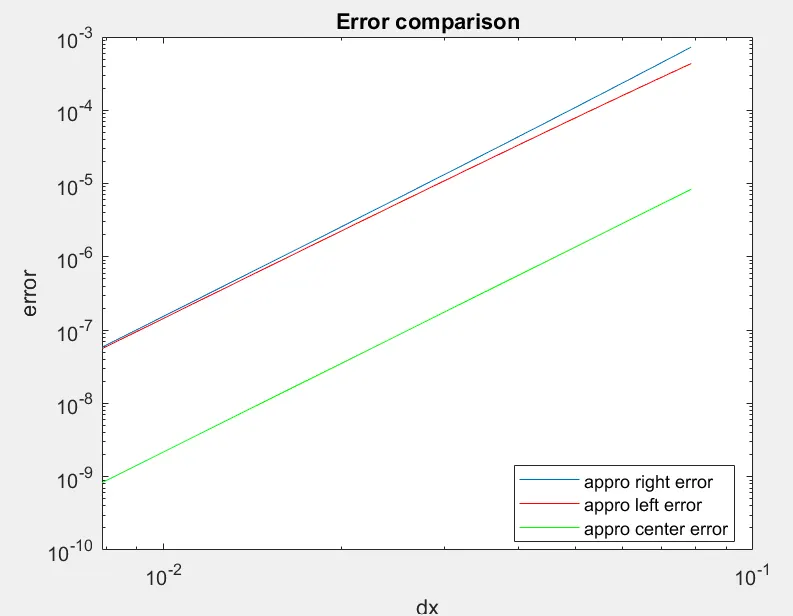
The skewed scheme works well when there isn't any points available on the sides of the grid. At this point, central scheme is not useful anymore.

The output plot gave us a graph that shows clearly that central difference scheme contains less error compared to the other schemes. It is why it's better to use CDS to solve equations, in order to obtain accurate results.