Week 7 - Simulation of a 1D Super-sonic nozzle flow simulation using Macormack Method
FLOW THROUGH A NOZZLE:
In practical we cannot compute the pattern of the flow of info in anozzle .so,we employ maccormack method of isentropic quasi static flow in anozzle .
Nozzle diagram with sections:
Since the problem setup is 1D, we consider only distribution in x-axis. Here Nozzle can be split into two sections
- Convergent Section
- Divergent Section
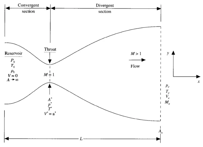
In solving all the necessary parameters,we use momentum,continuity,energy equations tosolve those.
Governing equations
These aare the partial differential time and space variables.
Conservative Form :
(i) Continutiy equation:
`(del(rho'A'))/(delt') + (del(rho'A'V'))/(delx') = 0`
(ii) Momentum equation:
`(del(rho'A'V'))/(delt') + (del(rho'A'V'^2+1/gammap'A'))/(delx')=1/gammap'(delA')/(delx')`
(iii) Energy equation ::
`(del[rho'((T')/(gamma-1)+gamma/2V'^2)A'])/(delt') + (del[rho'((T')/(gamma-1) +gamma/2V'^2)V'A' + p'A'V'])/(delx') = 0`
Non Conservative form :
(i) Continuity equation
`(partial rho)/(partial t) =rho'(partial V')/(partial x)`-`rho'V' (partial(lnA)/(partialx')) - V'(partialp')/(partialx')`
(ii) Momentum equation :::
`(partial V')/(partial t') = V'(partialV')/(partial x') - (1/gamma) [(partial T')/(partialx') +(T')/(rho') (partial rho')/(partialx')]`
(iii) Energy equation :::
`(partialT')/(partialt') = V'(partialT')/(partial x') - (gamma -1)T' [(partial V')/(partialx') +V' ( partial(ln(A))/ (partial x')]`
non dimensionless quantities:
Non dimensional temperature : `T'=T/T_0`
Non dimensional density : `rho'=rho/rho_0`
Non dimensional velocity : `V'=V/a_0`
Non dimensional distance :`x'=x/L`
Non dimensional time :`t'=t/(L/a_0)`
Non dimensional area = `A'=A/A_**`
MAIN PROGRAM:
close all
clear all
clc
n = 31;
L = 3;
x = linspace(0,L,n);
cfl = 0.5;
th = ((n-1)/2)+2;
nt = 1400;
tic
[v_nc,rho_nc,T_nc,mass_nc,M_nc,p_nc,v_throat_nc,rho_throat_nc,T_throat_nc,mass_throat_nc,M_throat_nc,p_throat_nc] = nonconservative();
Non_conservative_simulation_time = toc;
tic
[v_c,rho_c,T_c,mass_c,M_c,p_c,v_throat_c,rho_throat_c,T_throat_c,mass_throat_c,M_throat_c,p_throat_c]=conservative();
%Calculating the simulation time
conservative_simulation_time = toc;
%Analatical Solution Steady State
rho_an = 0.634*ones(1400);
T_an = 0.833*ones(1400);
p_an = 0.528*ones(1400);
M_an = 1*ones(1400);
figure(5)
a1 = subplot(4,1,1);
plot(linspace(1,nt,nt),rho_throat_nc);
hold on
plot(linspace(1,nt,nt),rho_throat_c,'g');
hold on
plot(linspace(1,nt,nt),rho_an,'k');
hold on
grid on
ylabel('Density')
legend('Non-conservative','Conseravative ','normal')
title('Variation in parameter at throat w.r.t time step')
a2 = subplot(4,1,2);
plot(linspace(1,nt,nt),T_throat_nc);
hold on
plot(linspace(1,nt,nt),T_throat_c);
hold on
plot(linspace(1,nt,nt),T_an);
hold on
grid on
ylabel('Temperature')
legend('Non-conservative','Conseravative','normal')
title('Variation in parameter at throat w.r.t time step')
a3 = subplot(4,1,3);
plot(linspace(1,nt,nt),p_throat_nc);
hold on
plot(linspace(1,nt,nt),p_throat_c);
hold on
plot(linspace(1,nt,nt),p_an);
hold on
grid on
ylabel('Pressure')
legend('Non-conservative','Conseravative','normal')
title('Variation in parameter at throat w.r.t time step')
a4 = subplot(4,1,4);
plot(linspace(1,nt,nt),M_throat_nc);
hold on
plot(linspace(1,nt,nt),M_throat_c);
hold on
plot(linspace(1,nt,nt),M_an);
hold on
grid on
ylabel('Mach number')
legend('Non-conservative','Conseravative','normal')
title('Variation in parameter at throat w.r.t time step')
figure(6)
b1 = subplot(4,1,1);
plot(x,rho_nc);
hold on
plot(x,rho_nc,'r');
hold on
grid on
ylabel('Density')
legend('Non-conservative','Conseravative','normal')
title('Variation in properties along X')
b2 = subplot(4,1,2);
plot(x,T_nc);
hold on
plot(x,T_nc,'b');
hold on
grid on
ylabel('Temperature')
legend('Non-conservative','Conseravative')
title('Variation in properties along X')
b3 = subplot(4,1,3);
plot(x,p_nc);
hold on
plot(x,p_nc,'g');
hold on
grid on
ylabel('Pressure')
legend('Non-conservative','Conseravative')
b4 = subplot(4,1,4);
plot(x,M_nc);
hold on
plot(x,M_nc,'b');
hold on
grid on
ylabel('Mach Number')
legend('Non-conservative','Conseravative')
figure(7)
plot(x,mass_nc)
hold on
plot(x,mass_c,'g')
hold on
plot(x,linspace(0.579,0.579,n),'k')
hold on
ylabel('non-dimentionless mass flow rate')
legend('Non-conservative approch','Conseravative approach','normal approach')
title('non-dimentionless mass flow rate comparision')
axis([0 3 0.55 0.6])
grid on
y = [rho_nc(th) rho_c(th) 0.634; T_nc(th) T_c(th) 0.833; p_nc(th) p_c(th) 0.528; M_nc(th) M_c(th) 1];
x_axis = categorical({'1.denisty','2.Temperature','3.Pressure','4.mach number'});
figure(8)
label= {'Non-conservative','Conseravative','normal'};
b = bar(x_axis,y,'group');
legend(label,'location','northoutside','Orientation','Vertical')
a = (1:size(y,1)).';
x_ax = [a-0.25 a a+0.25];
for k = 1:size(y,1)
 for m = 1:size(y,2)

text(x_ax(k,m),y(k,m),num2str(y(k,m),'%0.2f'),'HorizontalAlignment','center','VerticalAlignment','bottom')
 end
end
CONSERVATIVE FUNCTION
function[v,rho,T,mass,M,p,v_throat,rho_throat,T_throat,mass_throat,M_throat,p_throat]=conservative()
% geometry
L=3;
n=31;
x=linspace(0,L,n);
dx= x(2)-x(1);
%Initial Conditions
a=1+2.2*(x-1.5).^2;
th=find(a==1); %thraot node.
rho_initial=ones(1,n);
T_initial=ones(1,n);
for i= 1:n
 if (x(i)<=0.5)
 rho_initial(i)=1;
 T_initial(i)=1;
 elseif (x(i)>=0.5 && x(i)<=1.5)
 rho_initial(i)=1-0.366*(x(i)-0.5);
 T_initial(i)=1-0.167*(x(i)-0.5);
 elseif (x(i)>=1.5 && x(i)<=3)
 rho_initial(i)=0.634-0.3879*(x(i)-1.5);
 T_initial(i)=0.833-0.3507*(x(i)-1.5);
 end
end
v = 0.59./(rho_initial.*a);
gamma=1.4;
%Solution term
p= rho_initial.*T_initial;
u1 = rho_initial.*a;
u2 = rho_initial.*a.*v;
u3 = u1.*((T_initial/(gamma-1))+(0.5*gamma*v.^2));
%Time Step calculation based on Courant number.
cfl=0.5;
dt = min(cfl.*(dx./((sqrt(T_initial))+v)));
%Number of iterations
nt=1400;
rho=rho_initial;
T= T_initial;
%time loop
for k=1:nt

 %copy of solution terms
 u1old=u1;
 u2old=u2;
 u3old=u3;


 %Flux terms

 f1= u2;
 term=(((gamma-1)/gamma)*(u3-((gamma/2)*((u2.^2)./u1))));
 f2=((u2.^2)./u1)+ term;
 f3 = ((gamma*u2.*u3)./u1)-(gamma*(gamma-1)*(u2.^3))./(2*u1.^2);

 %predictor step
 for i =2:n-1
 df1dx(i)=(f1(i+1)-f1(i))/dx;
 df2dx(i)=(f2(i+1)-f2(i))/dx;
 df3dx(i)=(f3(i+1)-f3(i))/dx;
 dlogadx(i) = (log(a(i+1))-log(a(i)))/dx;

 dadx(i) = (a(i+1)-a(i))/dx;
 j2(i)=(1/gamma)*rho(i)*T(i)*dadx(i);

 %continuity equation
 du1dt_p(i)= -df1dx(i);
 %momentum equation
 du2dt_p(i)= -df2dx(i)+j2(i);
 %energy equation.
 du3dt_p(i)= -df3dx(i);

 %solution update.
 u1(i)=u1(i)+du1dt_p(i)*dt;
 u2(i)=u2(i)+du2dt_p(i)*dt;
 u3(i)=u3(i)+du3dt_p(i)*dt;
 end

 %primitive variables
 rho = u1./a;
 v = u2./u1;
 T= (gamma-1)*((u3./u1)-((gamma*v.^2)/2));

 %flux terms before corrector step
 f1= u2;
 term=(((gamma-1)/gamma)*(u3-(gamma*u2.^2)./(2*u1)));
 f2=((u2.^2)./u1)+ term;
 f3 = ((gamma*u2.*u3)./u1)-((gamma*(gamma-1)/2)*((u2.^3)./(u1.^2)));


 %corrector method
 for i=2:n-1
 df1dx(i)=(f1(i)-f1(i-1))/dx;
 df2dx(i)=(f2(i)-f2(i-1))/dx;
 df3dx(i)=(f3(i)-f3(i-1))/dx;
 dlogadx(i) = (log(a(i+1))-log(a(i)))/dx;
 dadx(i) = (a(i)-a(i-1))/dx;
 j2(i)=(1/gamma)*rho(i)*T(i)*dadx(i);

 %continuity equation
 du1dt_c(i)= -df1dx(i);
 %momentum equation
 du2dt_c(i)= -df2dx(i)+j2(i);
 %energy equation
 du3dt_c(i)= -df3dx(i);
 end

 %avergae derivative
 du1dt = 0.5*(du1dt_c+du1dt_p);
 du2dt = 0.5*(du2dt_c+du2dt_p);
 du3dt = 0.5*(du3dt_c+du3dt_p);

 %final solution update.
 for j =2:n-1
 u1(j)=u1old(j)+du1dt(j)*dt;
 u2(j)=u2old(j)+du2dt(j)*dt;
u3(j)=u3old(j)+du3dt(j)*dt;
 end

 %boundary conditions
 %inlet condition
 u1(1) = rho(1)*a(1);
 u2(1)= 2*u2(2)-u2(3);
 v(1) = u2(1)/u1(1);
 u3(1)= u1(1)*((T(1)/(gamma-1))+(0.5*gamma*v(1)^2));

 % outle Boundary
 u1(n) = 2*u1(n-1)-u1(n-2);
 u2(n) = 2*u2(n-1)-u2(n-2);
 u3(n) = 2*u3(n-1)-u3(n-2);

 %primitive terms
 rho = u1./a;
 v = u2./u1;
 T= (gamma-1)*((u3./u1)-(gamma/2)*(v.^2));

 %properties
 mass = rho.*a.*v;
 M = v./((T).^0.5);
 p= rho.*T;

 %throat values
 rho_throat(k)=rho(th);
 v_throat(k)=v(th);
 T_throat(k)=T(th);
 M_throat(k)=M(th);
 p_throat(k)=p(th);
 mass_throat(k)=mass(th);

 %residues at throat.
 u1_res(k)=du1dt(th);
 u2_res(k)=du2dt(th);
 u3_res(k)=du3dt(th);
%plotting the results
% plotting mass flow rate at different time steps
figure(2);
nt=1400;
plot(x, mass,'m', 'linewidth', 1.5)
grid on
ylabel('mass flow rate');
xlabel('nozzle length (x)');
title('mass flow rate at different time steps conservative appraoch');
legend

end
figure(4)
plot(linspace(1,nt,nt),u1_res);
hold on
plot(linspace(1,nt,nt),u2_res,'g');
hold on
plot(linspace(1,nt,nt),u3_res,'k');
grid on
ylabel('residues');
xlabel('timestep');
legend('u1plot','u2plot','u3plot');
title('residual plot');
end
NON CONSERVATIVE MACORMACK
function[v,rho,T,mass,M,p,v_throat,rho_throat,T_throat,mass_throat,M_throat,p_throat]=nonconservative()
%inputs
n=31;
x=linspace(0,3,n);
dx=x(2)-x(1);
%conidtions
rho=1-0.3146*x;
T=1-0.2314*x;
v=(0.1+1.09*x).*T.^0.5;
a=1+2.2*(x-1.5).^2;
th=find(a==1);
gamma=1.4;
%time steps
%Time Step calculation based on Courant number.
cfl=0.5;
dt = min(cfl.*(dx./((sqrt(T))+v)));
%Number of iterations
nt=1400;
%rho_initial=rho;
%T_initial=T;
%v_initial=v;
for k=1:nt
%copy of the variables
rho_old=rho;
T_old=T;
v_old=v;

%predictor step
 for j= 2:n-1
 dv_dx= (v(j+1)-v(j))/dx;
 drho_dx =(rho(j+1)-rho(j))/dx;
 dTdx = (T(j+1)-T(j))/dx;
 da_dx =(log(a(j+1))-log(a(j)))/dx;
 %continuity
 drhodt_p(j) = -rho(j)*dv_dx - rho(j)*v(j)*da_dx - v(j)*drho_dx;
 %momentum
 dvdt_p(j) = -v(j)*dv_dx - (1/gamma)*(dTdx+(T(j)/rho(j))*drho_dx);
 %energy
 dTdt_p(j) = -v(j)*dTdx -(gamma-1)*T(j)*(dv_dx+v(j)*da_dx);
 %solution updates
 v(j)= v(j)+dvdt_p(j)*dt;
 T(j)= T(j)+dTdt_p(j)*dt;
 rho(j)= rho(j)+drhodt_p(j)*dt;
 end

 % corrector Method
 for j= 2:n-1
 dv_dx= (v(j)-v(j-1))/dx;
 drho_dx =(rho(j)-rho(j-1))/dx;
 dTdx = (T(j)-T(j-1))/dx;
 da_dx =(log(a(j))-log(a(j-1)))/dx;
 %continuity
 drhodt_c(j) = -rho(j)*dv_dx-rho(j)*v(j)*da_dx-v(j)*drho_dx;
 %momentum
 dvdt_c(j) = -v(j)*dv_dx-(gamma^-1)*(dTdx+(T(j)/rho(j))*drho_dx);
 %energy
 dTdt_c(j) = -v(j)*dTdx -(gamma-1)*T(j)*(dv_dx+v(j)*da_dx);
 end

 %average
 dvdt_avg=0.5*(dvdt_c+dvdt_p);
 drhodt_avg = 0.5*(drhodt_c+drhodt_p);
 dTdt_avg = 0.5*(dTdt_p+dTdt_c);

 % Solution update
 for i =2:n-1
 v(i)= v_old(i)+dvdt_avg(i)*dt;
 T(i)= T_old(i)+dTdt_avg(i)*dt;
 rho(i)= rho_old(i)+drhodt_avg(i)*dt;
 end

 %Inlet condition by interpolation
 v(1)=2*v(2)-v(3);
 %outlet condition by interpolation
 v(n)=2*v(n-1)-v(n-2);
 T(n)=2*T(n-1)-T(n-2);
 rho(n)=2*rho(n-1)-rho(n-2);

 %properties
 mass = rho.*a.*v; M = v./((T).^0.5);
 p= rho.*T;

 %throat values
 rho_throat(k)=rho(th);
 v_throat(k)=v(th);
 T_throat(k)=T(th);
 M_throat(k)=M(th);
 p_throat(k)=p(th);
 mass_throat(k)=mass(th);

 %residues at throat.
 v_res(k)=dvdt_avg(th);
 rho_res(k)=drhodt_avg(th);
 T_res(k)=dTdt_avg(th);

%plotting the results
% plotting mass flow rate at different time steps
figure(1)
nt=1400;
plot(x, mass,'m', 'linewidth', 1.5)
grid on
ylabel('mass flow rate');
xlabel('nozzle length (x)');
title('mass flow rate at different time steps Non conservative approach');

end
figure(3)
plot(linspace(1,nt,nt),v_res);
hold on
plot(linspace(1,nt,nt),rho_res,'g');
hold on
plot(linspace(1,nt,nt),T_res,'k');
grid on
ylabel('residues');
xlabel('timestep');
legend('vplot','rhoplot','Tplot');
title('residual plot');
end
PLOTS:
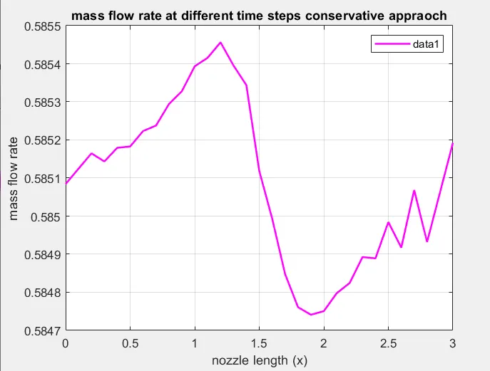
conservative macormack iteration
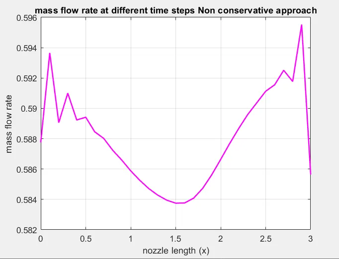
non consservative macormack iteration
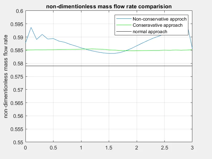
conservative vs non coservative vs normal (dimensionless Q)
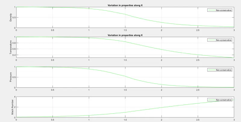
variation of patameters inside the nozzle
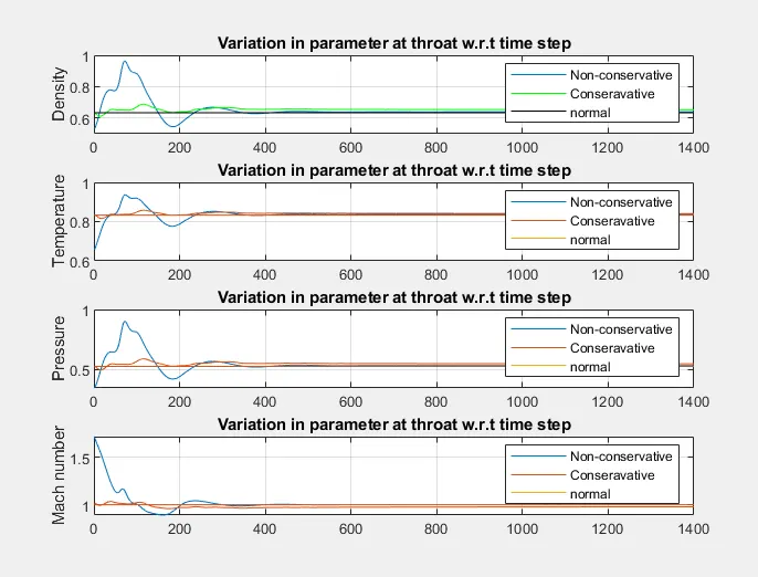
IT implies that non conservative are not not as stable as conservative.however,both tend stable at the end.
variation of parameters
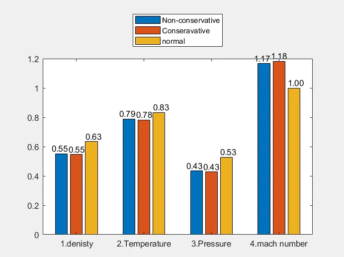
both conservative and non conservative nozzle flow are in same fashion.
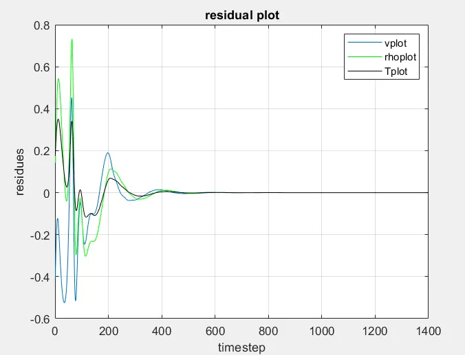
residual plot for non conservative
residual plot for consearvative
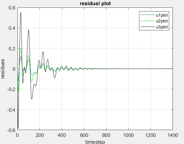
RESULT:conservative forms converges earlier than non consservative.This is because of quicker attaining of stabe solutionfrom the initial time.