Week 5.1 - Mid term project - Solving the steady and unsteady 2D heat conduction problem
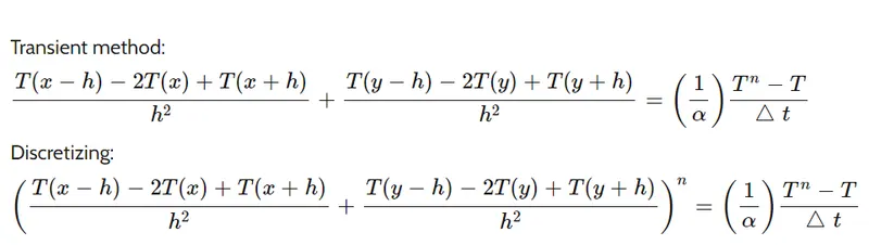
2D heat conduction equation
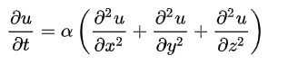
`alpha` coefficient of diffusivity
we start with temperature dependency equation and we then fiscitize it and we simply the equation 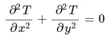
we descritise the above equation in all cases based on dependency using central difference formule
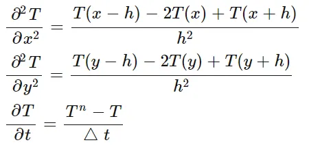
or

STEADY STATE ANALYSYS
IMPLICIT-JACOBI
steady state is an analysis for obtaining solution where we deal with the convection distibution over a meshhing.
implicit is an approach of getting solution at a particulartime rather than obtaining values from previous or next time steps.

clear all
close all
clc
nx=10;
ny=nx;
x=linspace(0,1,nx);
y=linspace(0,1,ny);
dx=x(2)-x(1);
dy=dx;
err=9e9;
tol=1e-4;
lt=400;
tt=600;
rt=800;
bt=900;
t=100*ones(nx,ny);
t(:,1)=400;
t(:,end)=800;
t(end,:)=600;
t(1,:)=900;
%calculating temperature at corners
t(1,1)=(tt+lt)/2;
t(nx,ny)=(rt+bt)/2;
t(1,ny)=(tt+rt)/2;
t(nx,1)=(lt+bt)/2;
t_prev=t;
t_old=t;
k=2*((dx^2+dy^2)/(dx^2*dy^2));

 %sTEADY JACOBI
while err > tol
    for i=2:nx-1
        for j=2:ny-1
            t(i,j)=(t_old(i-1,j)+t_old(i+1,j))/(k*(dx^2))+(t_old(i,j-1)+t_old(i,j+1))/(k*(dy^2));
        end
    end
     %updating
    error=max(max(abs(t_old-t)));
    t_old=t;


    figure(1)
    contourf(x,y,t)
    clabel(contourf(x,y,t))
    colorbar
    colormap(jet)
    set(gca,'ydir','reverse')
    xlabel('x')
    ylabel('y ')
end
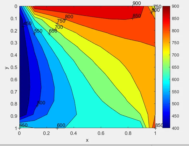
PLOT:
STEADY-IMPLLICIT GAUSS SEIDEL
in gauss seidel we use the new calculated values after first iteration.

CODE
clear all
close all
clc
nx=10
ny=nx
x=linspace(0,1,nx)
y=linspace(0,1,ny)
dx=x(2)-x(1)
dy=dx
err=9e9
tol=1e-4
lt=400;
tt=600;
rt=800;
bt=900;
t=100*ones(nx,ny);
t(:,1)=400;
t(:,end)=800;
t(end,:)=600;
t(1,:)=900;
k=2*((dx^2+dy^2)/(dx^2*dy^2));
%calculating temperature at corners
t(1,1)=(tt+lt)/2;
t(nx,ny)=(rt+bt)/2;
t(1,ny)=(tt+rt)/2;
t(nx,1)=(lt+bt)/2;
t_prev=t;
t_old=t;
%STEADY GAUSS
k=2*((dx^2+dy^2)/(dx^2*dy^2));

    while err > tol
    for i=2:nx-1
        for j=2:ny-1
            t(i,j)=(((t(i-1,j)+t_old(i+1,j))/dx^2)+((t(i,j-1)+t_old(i,j+1))/dy^2))/k;
        end
    end
     %updating
    error=max(max(abs(t_old-t)));
    t_old=t;

    figure(2)
    contourf(x,y,t)
    clabel(contourf(x,y,t))
    colorbar
    colormap(jet)
    set(gca,'ydir','reverse')
    xlabel('x')
    ylabel('y')
    pause(0.03)
    end
PLOT:
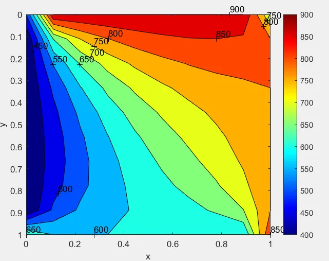
STEADY STATE -SOR-IMPLICIT:

ω-SOR CONSTANT.
CODE
clear all
close all
clc
nx=50
ny=nx
x=linspace(0,1,nx)
y=linspace(0,1,ny)
dx=x(2)-x(1)
dy=dx
err=9e9
tol=1e-4
lt=400
tt=600
rt=800
bt=900
t=100*ones(nx,ny)
t(:,ny)=600;
t(1,:)=900;
t(:,1)=400;
t(:,nx)=800;
%calculating temperature at corners
t(1,1)=(tt+lt)/2;
t(nx,ny)=(rt+bt)/2;
t(1,ny)=(tt+rt)/2;
t(nx,1)=(lt+bt)/2;
t_prev=t;
t_old=t;
%STEADY SOR
W=1.2
itsol=3
if itsol == 3
    itsor=0;
    while err > tol
        for i=2:nx-1
            for j=2:ny-1
                t(i,j)=W*(0.25*(t(i-1,j)+t_old(i+1,j)+t(i,j-1)+t_old(i,j+1)))+(1-W)*t_old(i,j);
            end
        end
        err=max(max(abs(t_old-t)));
        t_old=t;
        itsor=itsor+1;
    end
end
    figure(3)
    contourf(x,y,t)
    clabel(contourf(x,y,t))
    colorbar
    colormap(jet)
    set(gca, 'ydir' , 'reverse')
    xlabel('x')
    ylabel('y ')
PLOT:
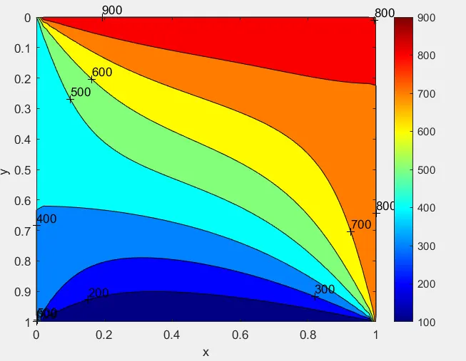
UNSTEADY OR TRANSIENT STATE--IMPLICIT
unstseady or transient state is one in which ,we get values based on time marching by mutual info flow.
JACOBI
IN UNSTEADY THE FORMULATED APPROACH IS SAME BUT WE WE USE TIME MARCHING .
for given no of time steps
tm1=1/(1+(2*k1)+(2*k2));
tm2=k1*tm1;
tm3=k2*tm1;
H=(t_old(i-1,j))+(t_old(i+1,j));
V=(t_old(i,j-1))+(t_old(i,j+1));
t(i,j)=(t_prev(i,j)*tm1)+(H*tm2)+(V*tm3);
we then using looping conditions,update the old and previous values.
CODE
clear all
close all
clc
nx=10
ny=nx
x=linspace(0,1,nx)
y=linspace(0,1,ny)
dx=x(2)-x(1)
dy=dx
err=9e9
tol=1e-4
lt=400
tt=600
rt=800
bt=900
t=100*ones(nx,ny)
t(:,1)=400;
t(:,end)=800;
t(end,:)=600;
t(1,:)=900;

%calculating temperature at corners
t(1,1)=(tt+lt)/2;
t(nx,ny)=(rt+bt)/2;
t(1,ny)=(tt+rt)/2;
t(nx,1)=(lt+bt)/2;
t_prev=t;
t_old=t;
alpha=1.1;
dt=0.01;
k1=alpha*(dt/dx^2);
k2=(alpha*(dt)/dy^2);
nt=1400;
for k=1:nt
    while err > tol
        for i=2:nx-1
            for j=2:ny-1
                tm1=1/(1+(2*k1)+(2*k2));
                tm2=k1*tm1;
                tm3=k2*tm1;
                H=(t_old(i-1,j))+(t_old(i+1,j));
                V=(t_old(i,j-1))+(t_old(i,j+1));
                t(i,j)=(t_prev(i,j)*tm1)+(H*tm2)+(V*tm3);
            end
        end
      err=max(max(abs(t_old-t)));
      t_old=t;
    end
    t_prev=t;
end
    figure(4)
    contourf(x,y,t)
    clabel(contourf(x,y,t))

    colormap(jet)
    set(gca, 'ydir' , 'reverse')
    xlabel('x')
    ylabel('y ')
PLOT
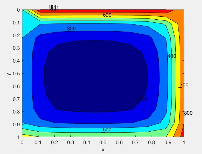
UNSTEADY(TRANSIENT)-GAUSS SEIDEL
for given number of time steps
tm1=1/(1+(2*k1)+(2*k2));
tm2=k1*tm1;
tm3=k2*tm1;
H=(t_old(i-1,j))+(t_old(i+1,j));
V=(t_old(i,j-1))+(t_old(i,j+1));
t(i,j)=(t_prev(i,j)*tm1)+(H*tm2)+(V*tm3)
we then using looping conditions,update the old and previous valus.
CODE
clear all
close all
clc
nx=10
ny=nx
x=linspace(0,1,nx)
y=linspace(0,1,ny)
dx=x(2)-x(1)
dy=dx
err=9e9
tol=1e-4
lt=400
tt=600
rt=800
bt=900
t=100*ones(nx,ny)
t(:,ny)=600;
t(1,:)=900;
t(:,1)=400;
t(:,nx)=800;
%calculating temperature at corners
t(1,1)=(lt+tt)/2;
t(nx,ny)=(rt+bt)/2;
t(1,ny)=(tt+rt)/2;
t(nx,1)=(lt+bt)/2;
t_prev=t;
t_old=t;
alpha=1.1;
dt=0.01;
k1=alpha*(dt/dx^2);
k2=(alpha*(dt)/dy^2);
nt=1400;
for k=1:nt
    while err > tol
        for i=2:nx-1
            for j=2:ny-1
               tm1=1/(1+(2*k1)+(2*k2));
                tm2=k1*tm1;
                tm3=k2*tm1;
                H=(t_old(i-1,j))+(t_old(i+1,j));
                V=(t_old(i,j-1))+(t_old(i,j+1));
                t(i,j)=(t_prev(i,j)*tm1)+(H*tm2)+(V*tm3)
            end
        end
      err=max(max(abs(t_old-t)));
      t_old=t;
    end
    t_prev=t;
end
    figure(5)
    contourf(x,y,t)
    clabel(contourf(x,y,t))
    colorbar
    colormap(jet)
    set(gca, 'ydir' , 'reverse')
    xlabel('x')
    ylabel('y ')
PLOT
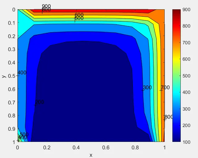
IMPLICIT SOR UNSTEADY(TRANSIENT)
for range of our time steps
tm1=1/(1+(2*k1)+(2*k2));
tm2=k1*tm1;
tm3=k2*tm1;
H=(t_old(i-1,j))+(t_old(i+1,j));
V=(t_old(i,j-1))+(t_old(i,j+1));
t(i,j)=(t_prev(i,j)*tm1)+(H*tm2)+(V*tm3)
we then using looping conditions,update the old and previous values
CODE
clear all
close all
clc
nx=10
ny=nx
x=linspace(0,1,nx)
y=linspace(0,1,ny)
dx=x(2)-x(1)
dy=dx
err=9e9
tol=1e-4
lt=400
tt=600
rt=800
bt=900
t=100*ones(nx,ny)
t(:,ny)=600;
t(1,:)=900;
t(:,1)=400;
t(:,nx)=800;
%calculating temperature at corners
t(1,1)=(tt+lt)/2;
t(nx,ny)=(rt+bt)/2;
t(1,ny)=(tt+rt)/2;
t(nx,1)=(lt+bt)/2;
t_prev=t;
t_old=t;
alpha=1.1;
dt=0.01;
W=1.1;
k1=alpha*(dt/dx^2);
k2=(alpha*(dt)/dy^2);
nt=1400;
for k=1:nt
    while err > tol
        for i=2:nx-1
            for j=2:ny-1
                tm1=1/(1+(2*k1)+(2*k2));
                tm2=k1*tm1;
                tm3=k2*tm1;
                H=(t(i-1,j))+(t_old(i+1,j));
                V=(t(i,j-1))+(t_old(i,j+1));
                t(i,j)=W*(t_prev(i,j)*tm1+tm2*H+tm3*V)+(1-W)*t_prev(i,j);

            end
        end
      err=max(max(abs(t_old-t)));
      t_old=t;
    end
    t_prev=t;
end
    figure(6)
    contourf(x,y,t)
    clabel(contourf(x,y,t))
    colorbar
    colormap(jet)
    set(gca, 'ydir' , 'reverse')
    xlabel('x')
    ylabel('y ')
PLOT
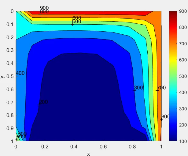
EXPLICIT--TRANSIENT
in explicit analysys ,we get data from previous or next time steps and we calculate at given time step.
CODE
clear all
close all
clc
nx=10
ny=nx
x=linspace(0,1,nx)
y=linspace(0,1,ny)
dx=x(2)-x(1)
dy=dx
dt=1e-3;
err=9e9
tol=1e-4
lt=400
tt=600
rt=800
bt=900
t=100*ones(nx,ny)
t(:,ny)=600;
t(1,:)=900;
t(:,1)=400;
t(:,nx)=800;
%calculating temperature at corners
t(1,1)=(tt+lt)/2;
t(nx,ny)=(rt+bt)/2;
t(1,ny)=(tt+rt)/2;
t(nx,1)=(lt+bt)/2;
t_prev=t;
t_old=t;
alpha=1.1;
W=1.1;
k1=alpha*(dt/dx^2);
k2=(alpha*(dt)/dy^2);
nt=1400;
stexp=0;
for k=1:nt

    while(err > tol)
        for i=2:nx-1
            for j=2:ny-1
                 tm1=t_old(i,j);
                 tm2=k1*(t_old(i+1,j)-2*t_old(i,j)+(t_old(i-1,j)));
                 tm3=k2*(t_old(i,j+1)-2*t_old(i,j)+t_old(i,j-1));
                 t(i,j)=tm1+tm2+tm3;
            end
        end
        err=max(max(abs(t_old-t)));
        t_old=t;
    end
end
figure(7)
    contourf(x,y,t)
    clabel(contourf(x,y,t))
    colorbar
    colormap(jet)
    set(gca,'ydir','reverse')
    xlabel('x')
    ylabel('y ')
PLOT:
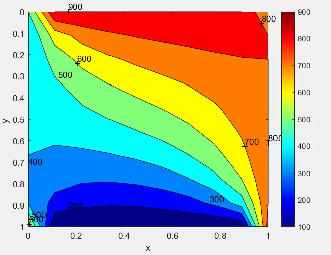
conclusion:
1.SOR is an hybrid chnique where the results are quick as it taakes less no of iterations.
2.explicit schemes are more faster than implicit because its time marching type with dependency of values of values in other time steps.
3.implicit schemes are bit acccurate because wwe follow equational approach rather than time dominant approach-explicit.
4.steady state is accurate than unsteady similar to impllicit and explicit.