Aim: Simulation of a 1D Super-sonic nozzle flow simulation using Macormack Method.

Objective

• simulate the isentropic flow through a quasi 1D subsonic-supersonic nozzle using both the conservative and non-conservative form of the fluid flow equations

The following plots are to be shown in report

1. Steady-state distribution of primitive variables inside the nozzle
   2. Time-wise variation of the primitive variables
   3. Variation of Mass flow rate distribution inside the nozzle at different time steps during the time-marching process
   4. Comparison of normalized mass flow rate distributions of both forms

Expected Results:

Perform a grid independence test on the solution and explain all your findings.

The code must be modular. You need to write separate functions to solve both forms.

Discuss all the plots you are providing with observed inferences.

Note:

Refer CFD book by John Anderson for Initial and boundary conditions.

Description/Analysis

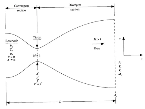
We consider the steady isentropic flow through a convergent-divergent nozzle as shown below. The flow at the inlet to the nozzle comes from a reservoir. The flow expands isentropically to supersonic speeds at the nozzle exit. The flow is locally subsonic at the convergent section of the nozzle, sonic at the throat and supersonic at the divergent section.

We assume 1d inviscid flow through the nozzle. Hence the resulting fluid flow equations to be converted to their algebraic form for the numerical solution of this problem are show below (reference pg 78 Section 2.8 Anderson).

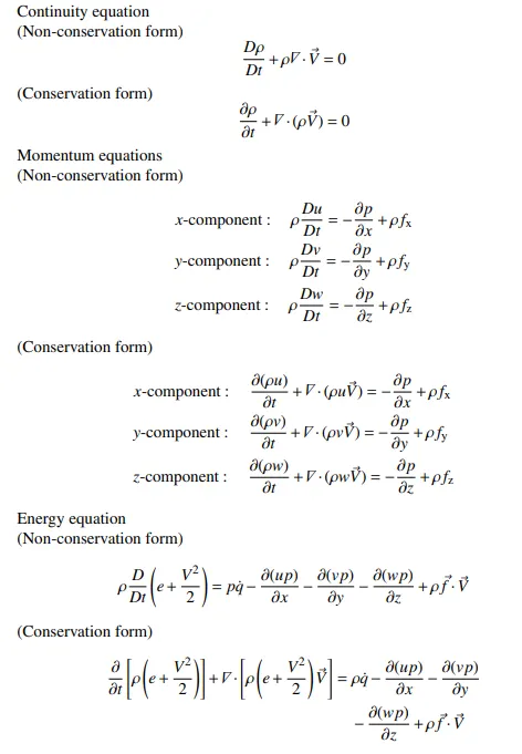
Solutions to these equations are obtained using McCormack’s method which is suitable for inviscid flow problems. It is a 2^nd order accurate explicit difference scheme in both the spatial and temporal components of the above fluid flow equations.

Initial Conditions/Boundary Conditions

Initial conditions should be chosen such that their values are close to that of the steady state solution. This would guarantee a faster time marching solution. Large deviations can lead to large gradients during the time marching procedure and hence make the solution go unstable.

For boundary conditions at the inflow side using the method of characteristics, we need to specify 2 flow field variables, density and temperature, as fixed with a third variable V for velocity as floating.

For boundary conditions at the outflow side due to supersonic conditions, all variables must float because the left and right running characteristics are both pointing out of the exit boundary and so all variables cannot be fixed.

Results/Discussion

Steady State Solution Comparison

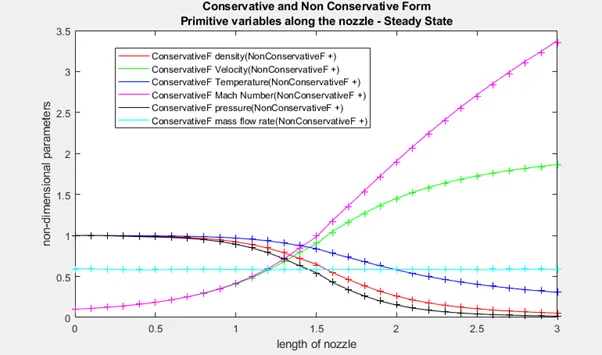
The following plot shows a comparison of the conservative and non-conservative form of the fluid flow equations to predict the steady state primitive variables along the length of the nozzle.

Both fluid flow forms are generating the same results along the nozzle and this is to be expected as the choice of conservative or non-conservative should not matter for the case of isentropic subsonic-supersonic flow through a nozzle. Only in the case of shock capturing does the choice of which fluid flow form matters which is outside the scope of this challenge.

Time-wise variation of flow variables.

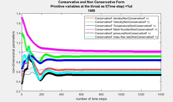
The following plot show the time-wise variation of the primitive variables for the 2 forms with steady values achieved approximately after 600 time steps.

The following plot shows the variation of mass flow rate along the nozzle at different time steps for the 2 forms.

For the non-conservative form we can see how at earlier time steps from nt=50-150 that the mass flow rate is quite unsteady. This is due to transient variations of the flow fields. However after 200 steps we see the mass flow rate stabilizing to a constant along the length of the nozzle which confirms our knowledge that the mass flow rate being the product of density*velocity *cross sectional area is a constant.

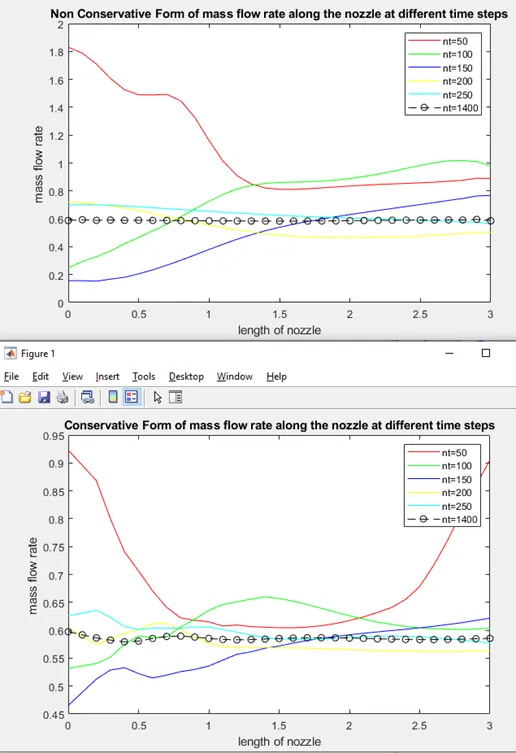
In the above plot, for the conservative form we see a milder variations of the mass flow rate due to the assumed initial condition. This is shown more clearly below for a time step of 1. Here the steady state mass flow distribution is much closer to the theoretical value (green) with little or no oscillation.

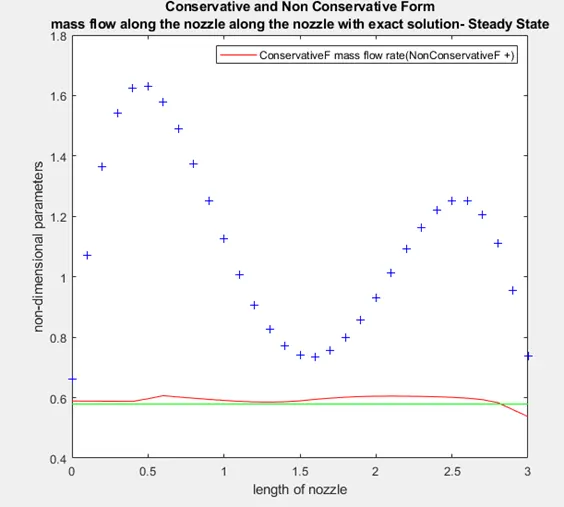
In the conservative form, the dependent variables (variables for which we directly calculate the numbers) are not the primitive variables. These primitive variables (rho, V, T and p) are decoded from the solutions vector (U1,U2,U3). This is also true for the mass flow rate. Ie, the mass flow itself is a dependent variable/primary result.

In contrast, the dependent variables in the non- conservative form are the primitive variables and hence the mass flow rate is obtained as a secondary result.

It is for those reasons outlined above that the conservative form calculates a more accurate mass flow rate along the nozzle length.

Grid Independence

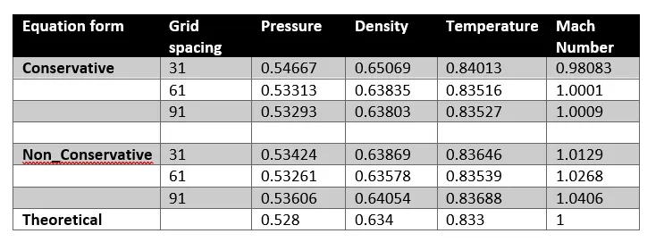
The table below shows the values predicted by the program and the corresponding analytical value. It seems that grid independence is achieved for grid values 61 and 91 for the conservative case and also for the non-conservative case. However, there is no superiority of either form over the other. Both cases yield satisfactory results.

In terms of programming effort, the conservative form requires additional scripting due to the fact that the primitive variables need to be decoded from the solution vector.

M file

clear all
close all
clc
%grid points along nozzle of total length 3
N=31;
N_throat=((N-1)/2+1);
x=linspace(0,3,N);
dx=x(2)-x(1);
g=1.4;
%time step
nt=1400;
C=0.5;

%run m file. 10 plots will appear. Please give it some time to complete.
[nt]=conservative_form(N,x,dx,g,nt,C,N_throat);
[nt]=non_conservative_form(N,x,dx,g,nt,C,N_throat); 

Conservative function

function [nt]=conservative_form(N,x,dx,g,nt,C,N_throat);
%% 

%pre-allocation
dU1dtp=ones();
dU2dtp=ones();
dU3dtp=ones();
dU1dtc=ones();
dU2dtc=ones();
dU3dtc=ones();
rho_c=ones();
rho_c_throat=ones();
V_throat=ones();
T_throat=ones();
M_throat=ones();
J2=ones();
NN=N_throat;


nt_array=1:nt; %for plotting
%initial conditions @t=0 eqn7.120a
for u=1:length(x)
    if (x(u) >=0) && (x(u) <=0.5)
        rho_c(u)=1;
        T(u)=1;
    elseif (x(u)> 0.5) && (x(u)<=1.5)
        rho_c(u)=1-0.366*(x(u)-0.5);
        T(u)=1-0.167*(x(u)-0.5);
    elseif (x(u) >1.5) && (x(u)<=3.5)
        rho_c(u)=0.634-0.3879*(x(u)-1.5);
        T(u)=0.833-0.3507*(x(u)-1.5); 
    end
end
%Initial Conditions
A=1+2.2*(x-1.5).^2;%area
%0.59 is chosen to stabilize solution eqn7.121-122c
U1=rho_c.*A;
V=0.59./U1;
U2=rho_c.*A.*V;
U3=rho_c.*((T./(g-1))+(g.*V.^2./2)).*A;
%general flow field variables
% p=rho_c.*T;
% M=V./(T.^0.5);
% m_dot=rho_c.*A.*V;


%dt must be less than, or at best equal to,
%the time it takes a sound wave to move from one grid point to the next.
%% 
%outer loop
for k=1:nt
    
    % find the minimum timestep for each and every timestep
    for i=1:N
    u=T(i).^0.5;% speed of sound eqn7.75
    dt_min(i)=C*(dx/(u+V(i)));
    end
    dt=min(dt_min)
    
    % need a copy of data at the start and end of time step for 
    %comparison purposes.
    U1_old=U1;
    U2_old=U2;
    U3_old=U3;
    
    F1=U2;
    F2= (U2.^2./U1) + ((g-1)/g).*(U3-((g/2)*(U2.^2./U1)));
    F3= (g.*U3.*U2./U1)-(g*(g-1)/2).*(U2.^3./U1.^2);
    
    
    %predictor method on the spatial derevatives
    for j=2:N-1 % 2: doing calc on inner nodes
      
      
        %source term - non pure form
        J2(j)=(1/g).*(rho_c(j).*T(j)).*((A(j+1)-A(j))/dx);
        
        %predictor method on the spatial derevatives
        dU1dtp(j)=-(F1(j+1)-F1(j))/dx;%Continuity
        dU2dtp(j)=-(F2(j+1)-F2(j))/dx+J2(j);%Momentum
        dU3dtp(j)=-(F3(j+1)-F3(j))/dx;%Energy

        %solution update: THis is placed inside of this loop to ensure correct
        %matrix sizes
        U1(j)=U1_old(j)+dU1dtp(j)*dt;
        U2(j)=U2_old(j)+dU2dtp(j)*dt;
        U3(j)=U3_old(j)+dU3dtp(j)*dt;   
        
    end
    
    %corrector method on the spatial derevatives   
    for j=2:N-1 % 2: doing calc on inner nodes      
        
        J2(j)=(1/g)*(rho_c(j)*T(j))*((A(j)-A(j-1))/dx);%source term non pure
        dU1dtc(j)=-(F1(j)-F1(j-1))/dx;%Continuity
        dU2dtc(j)=-(F2(j)-F2(j-1))/dx +J2(j); %MOmentum
        dU3dtc(j)=-(F3(j)-F3(j-1))/dx;%Energy
        %update flux terms
        F1=U2;
        F2=U2.^2./U1+((g-1)./g)*(U3-((g./2)*(U2.^2./U1)));
        F3=g.*U3.*U2./U1-(g*(g-1)/2)*(U2.^3./U1.^2);
          
    end
    
    %compute average time deriviative
    dU1dt=0.5*(dU1dtp+dU1dtc);
    dU2dt=0.5*(dU2dtp+dU2dtc);
    dU3dt=0.5*(dU3dtp+dU3dtc);
    
    %final solution update after the predictor and corrector steps
    for j=2:N-1
        U1(j)=U1_old(j)+dU1dt(j)*dt;
        U2(j)=U2_old(j)+dU2dt(j)*dt;
        U3(j)=U3_old(j)+dU3dt(j)*dt;
    end
    
    % apply boundary conditions eqn 7.119a
    %Inlet
    U1(1)=A(1)*rho_c(1);      %u = a*rho_c. rho_c was missing
    U2(1)=2*U2(2)-U2(3);
    U3(1)=U1(1)*((T(1)/(g-1))+(g/2)*(U2(1)/U1(1)).^2);
    %Outlet
    U1(N)=2*U1(N-1)-U1(N-2);
    U2(N)=2*U2(N-1)-U2(N-2);
    U3(N)=2*U3(N-1)-U3(N-2);
    
    
    rho_c=U1./A;
    V=U2./U1;
    T=(g-1).*((U3./U1) - ((g/2).*V.^2));
    p=rho_c.*T;
    M=V./(T.^0.5);
    %mass flow rate also =U2
    m_dot=rho_c.*A.*V;
   
   %for grid indpendence check
   %flow field variables at the throat
   if NN==N_throat
       rho_c_throat(k)=rho_c(NN);
       V_throat(k)=V(NN);
       T_throat(k)=T(NN);
       M_throat(k)=V_throat/T_throat.^0.5;
       p_throat=rho_c_throat.*T_throat;
       m_dot_throat=rho_c_throat.*V_throat;
   end
   
     figure(1)
     movegui(figure(1),'northwest');
    if k==50
        plot(x,m_dot,'r')
        hold on
    elseif k==100
        plot(x,m_dot,'g')
        hold on
    elseif k==150
        plot(x,m_dot,'b')
        hold on
    elseif k==200
        plot(x,m_dot,'y')
        hold on
    elseif k==250
        plot(x,m_dot,'c')
        hold on
    elseif k==nt
        plot(x,m_dot,'k--o')
        hold on
    xlabel('length of nozzle')
    ylabel('mass flow rate ')
    legend('nt=50','nt=100','nt=150','nt=200','nt=250','nt=1400');
    title('Conservative Form of mass flow rate along the nozzle at different time steps');
    end
   
end
%% 


   figure(2)
   movegui(figure(2),'north');
   plot(x,rho_c,'r')
   hold on
   plot(x,V,'g')
   plot(x,T,'b')
   plot(x,M,'m')
   plot(x,p,'k')
   plot(x,m_dot,'c')
   xlabel('length of nozzle')
   ylabel('non-dimensional parameters')
   legend('Conservative Form density',...
          'Conservative Form Velocity',...
          'Conservative Form Temperature',...
          'Conservative Form Mach Number',...
          'Conservative Form pressure',...
          'Conservative Form mass flow rate');
   title('Conservative Form of primitive variables along the nozzle - Steady State'); 

   
   figure(3)
   movegui(figure(3),'northeast');
   plot(nt_array,rho_c_throat,'r')
   hold on
   plot(nt_array,V_throat,'g')
   plot(nt_array,T_throat,'b')
   plot(nt_array,M_throat,'m')
   plot(nt_array,p_throat,'k')
   plot(nt_array,m_dot_throat,'c')
   xlabel('number of time steps')
   ylabel('non-dimensional parameters')
   legend('Conservative Form density','Conservative Form Velocity','Conservative Form Temperature','Conservative Form Mach Number',...
          'Conservative Form pressure','Conservative Form mass flow rate')
   title(sprintf('Conservative Form Primitive/Flow field Variables - Time step =%d',k'));
   
   figure(7)
   plot(x,rho_c,'r')
   hold on
   plot(x,V,'g')
   plot(x,T,'b')
   plot(x,M,'m')
   plot(x,p,'k')
   plot(x,m_dot,'c')
   xlabel('length of nozzle')
   ylabel('non-dimensional parameters')
   legend('Conservative Form density',...
          'Conservative Form Velocity',...
          'Conservative Form Temperature',...
          'Conservative Form Mach Number',...
          'Conservative Form pressure',...
          'Conservative Form mass flow rate');
   title('Conservative Form of primitive variable along the nozzle - Steady State'); 

   
   figure(8)
   plot(nt_array,rho_c_throat,'r')
   hold on
   plot(nt_array,V_throat,'g')
   plot(nt_array,T_throat,'b')
   plot(nt_array,M_throat,'m')
   plot(nt_array,p_throat,'k')
   plot(nt_array,m_dot_throat,'c')
   xlabel('number of time steps')
   ylabel('non-dimensional parameters')
   legend('Conservative Form density','Conservative Form Velocity','Conservative Form Temperature','Conservative Form Mach Number',...
          'Conservative Form pressure','Conservative Form mass flow rate')
   title(sprintf('Conservative Form Primitive/Flow field Variables - Time step =%d',k'));
   
   figure(9)
   plot(x,m_dot,'r')
   hold on
   xlabel('length of nozzle')
   ylabel('non-dimensional parameters')
   legend('Conservative Form mass flow rate');
   title('Conservative Form of mass flow rate along the nozzle - Steady State'); 

   
   figure(10)
   plot(nt_array,m_dot_throat,'r')
   hold on 
   xlabel('number of time steps')
   ylabel('non-dimensional parameters')
   legend('Conservative Form mass flow rate')
   title(sprintf('Conservative Form mass flow rate - Time step =%d',k'));


end

NonConservative Function

function [nt]=non_conservative_form(N,x,dx,g,nt,C,N_throat);
%% 
nt_array=1:nt; %for plotting
%initial conditions
rho=1-0.3146*x;
T=1-0.2314*x; % T temperature
V=((0.1+1.09*x)).*T.^0.5; % .* for element wise calcs
a=1+2.2*(x-1.5).^2; %area
rho_exact=0.579*ones(1,N);
NN=N_throat;

%dt must be less than, or at best equal to,
%the time it takes a sound wave to move from one grid point to the next.
%% 


%outer loop
for k=1:nt
    
    % find the minimum timestep for each and every timestep
    for i=1:N
    u=T(i).^0.5;% speed of sound eqn7.75
    dt_min(i)=C*(dx/(u+V(i)));
    end
    dt=min(dt_min)
    % need a copy of data at the start and end of time step for 
    %comparison purposes.
    rho_old=rho;
    V_old=V;
    T_old=T;
    
    
    %predictor method
    for j=2:N-1 % 2: doing calc on inner nodes
        dVdx=(V(j+1)-V(j))/dx;
        drhodx=(rho(j+1)-rho(j))/dx;
        dTdx=(T(j+1)-T(j))/dx;
        dlog_adx=(log(a(j+1))-log(a(j)))/dx;
        
        %continuity eqn
        drhodt_p(j)=-rho(j)*dVdx-rho(j)*V(j)*dlog_adx-V(j)*drhodx;
        
        %Momentum Eqn
        dVdt_p(j)=-V(j)*dVdx-(1/g)*(dTdx+(T(j)/rho(j))*drhodx);
        
        %Energy Eqn
        dTdt_p(j)=-V(j)*dTdx-(g-1)*T(j)*(dVdx+V(j)*dlog_adx);
        
        %solution update: THis is placed inside of this loop to ensure correct
        %matrix sizes
        rho(j)=rho(j)+drhodt_p(j)*dt;
        V(j)=V(j)+dVdt_p(j)*dt;
        T(j)=T(j)+dTdt_p(j)*dt;
    end
    
    %corrector method
    for j=2:N-1 % 2: doing calc on inner nodes
        dVdx=(V(j)-V(j-1))/dx;
        drhodx=(rho(j)-rho(j-1))/dx;
        dTdx=(T(j)-T(j-1))/dx;
        dlog_adx=(log(a(j))-log(a(j-1)))/dx;
        
        %continuity eqn
        drhodt_c(j)=-rho(j)*dVdx-rho(j)*V(j)*dlog_adx-V(j)*drhodx;
        
        %Momentum Eqn
        dVdt_c(j)=-V(j)*dVdx-(1/g)*(dTdx+(T(j)/rho(j))*drhodx);
        
        %Energy Eqn
        dTdt_c(j)=-V(j)*dTdx-(g-1)*T(j)*(dVdx+V(j)*dlog_adx);
        
    end
    
    %compute average time deriviative
    drhodt=0.5*(drhodt_p+drhodt_c);
    dVdt=0.5*(dVdt_p+dVdt_c);
    dTdt=0.5*(dTdt_p+dTdt_c);
    
    %final solution update after the predictor and corrector steps
    for i=2:N-1
    rho(i)=rho_old(i)+drhodt(i)*dt;
    V(i)=V_old(i)+dVdt(i)*dt;
    T(i)=T_old(i)+dTdt(i)*dt;
    end
    
    % apply boundary conditions
    
    %inlet velocity f(N)
    V(1)=2*V(2)-V(3);
    
   %outlet f(N)
   V(N)=2*V(N-1)-V(N-2);
   rho(N)=2*rho(N-1)-rho(N-2);
   T(N)=2*T(N-1)-T(N-2);
   
    %for grid indpendence check
    if NN==N_throat
       %flow field variables at the throat
       rho_throat(k)=rho(NN);
       V_throat(k)=V(NN);
       T_throat(k)=T(NN);
       M_throat(k)=V_throat/T_throat.^0.5;
       p_throat=rho_throat.*T_throat;
       %area at throat =1
       m_dot_throat=rho_throat.*V_throat;
    end
   
   %general flow field variables
   p=rho.*T;
   M=V./(T.^0.5);
   m_dot=rho.*a.*V;
   
          figure(4)
    movegui(figure(4),'southwest');
    if k==50
        plot(x,m_dot,'r')
        hold on
    elseif k==100
        plot(x,m_dot,'g')
        hold on
    elseif k==150
        plot(x,m_dot,'b')
        hold on
    elseif k==200
        plot(x,m_dot,'y')
        hold on
    elseif k==250
        plot(x,m_dot,'c')
        hold on
    elseif k==nt
        plot(x,m_dot,'k--o')
        hold on
    xlabel('length of nozzle')
    ylabel('mass flow rate ')
    legend('nt=50','nt=100','nt=150','nt=200','nt=250','nt=1400');
    title('Non Conservative Form of mass flow rate along the nozzle at different time steps');
    end
   

   
end
%% 


   %spatial dependence of flow field variables.
   figure(5)
   movegui(figure(5),'south');
   plot(x,rho,'r')
   hold on
   plot(x,V,'g')
   plot(x,T,'b')
   plot(x,M,'m')
   plot(x,p,'k')
   plot(x,m_dot,'c')
   xlabel('length of nozzle')
   ylabel('non-dimensional parameters')
   legend('NonConservativeF density',...
          'NonConservativeF Velocity',...
          'NonConservativeF Temperature',...
          'NonConservativeF Mach Number',...
          'NonConservativeF pressure',...
          'NonConservativeF mass flow rate');
   title({' Non Conservative Form',...
          'Primitive variables along the nozzle - Steady State'});



   %time dependent variations of the flow fields variables at the throat
   figure(6)
   movegui(figure(6),'southeast');
   plot(nt_array,rho_throat,'r')
   hold on
   plot(nt_array,V_throat,'g')
   plot(nt_array,T_throat,'b')
   plot(nt_array,M_throat,'m')
   plot(nt_array,p_throat,'k')
   plot(nt_array,m_dot_throat,'c')
   xlabel('number of time steps')
   ylabel('non-dimensional parameters')
   legend('NonConservative Form Density',...
          'NonConservative Form Velocity',...
          'NonConservative Form Temperature',...
          'NonConservative Form Mach Number',...
          'NonConservative Form Pressure',...
          'NonConservative Form mass flow rate');
   title({'Non Conservative Form',...
          'Primitive variables at the throat as f(Time step) =%d',k'});
   
  

   figure(7)
   movegui(figure(7),'center');
   plot(x,rho,'+r')
   hold on
   plot(x,V,'+g')
   plot(x,T,'+b')
   plot(x,M,'+m')
   plot(x,p,'+k')
   plot(x,m_dot,'+c')
   xlabel('length of nozzle')
   ylabel('non-dimensional parameters')
   legend('ConservativeF density(NonConservativeF +)',...
          'ConservativeF Velocity(NonConservativeF +)',...
          'ConservativeF Temperature(NonConservativeF +)',...
          'ConservativeF Mach Number(NonConservativeF +)',...
          'ConservativeF pressure(NonConservativeF +)',...
          'ConservativeF mass flow rate(NonConservativeF +)');
   title({'Conservative and Non Conservative Form',...
          'Primitive variables along the nozzle - Steady State'});

   figure(8)
   movegui(figure(8),'center');
   plot(nt_array,rho_throat,'+r','marker','+','MarkerIndices',1:5:length(rho_throat))
   hold on
   %plot(nt_array,V_throat,'+g','marker','+','MarkerIndices',1:5:length(V_throat))
   plot(nt_array,V_throat,'+g')
   plot(nt_array,T_throat,'+b')
   plot(nt_array,M_throat,'+m')
   plot(nt_array,p_throat,'+k')
   plot(nt_array,m_dot_throat,'+c')
   xlabel('number of time steps')
   ylabel('non-dimensional parameters')
   legend('ConservativeF density(NonConservativeF +)',...
          'ConservativeF Velocity(NonConservativeF +)',...
          'ConservativeF Temperature(NonConservativeF +)',...
          'ConservativeF Mach Number(NonConservativeF +)',...
          'ConservativeF pressure(NonConservativeF +)',...
          'ConservativeF mass flow rate(NonConservativeF +)');
   title({'Conservative and Non Conservative Form',...
          'Primitive variables at the throat as f(Time step) =%d',k'});
      
   figure(9)
   movegui(figure(9),'center');
   plot(x,m_dot,'+b')
   hold on 
   plot(x,rho_exact,'g');
   xlabel('length of nozzle')
   ylabel('non-dimensional parameters')
   legend('ConservativeF mass flow rate(NonConservativeF +)');
   title({'Conservative and Non Conservative Form',...
          'mass flow along the nozzle along the nozzle with exact solution- Steady State'});

   figure(10)
   movegui(figure(10),'center');
   plot(nt_array,m_dot_throat,'+b','marker','+','MarkerIndices',1:5:length(m_dot_throat))
   xlabel('number of time steps')
   ylabel('non-dimensional parameters')
   legend('ConservativeF mass flow rate(NonConservativeF +)');
   title({'Conservative and Non Conservative Form',...
          'mass flow at the throat as f(Time step) =%d',k'});

end